
Active learning
Active learning inverts the usual order. Instead of generating a dataset and then training, the model trains, decides where it is least certain, asks for labels there, trains again. When a label costs a finite-element solve, choosing which solves to run is the whole game.
physicsnemo.active_learning is the bundled framework for that loop.
The loop
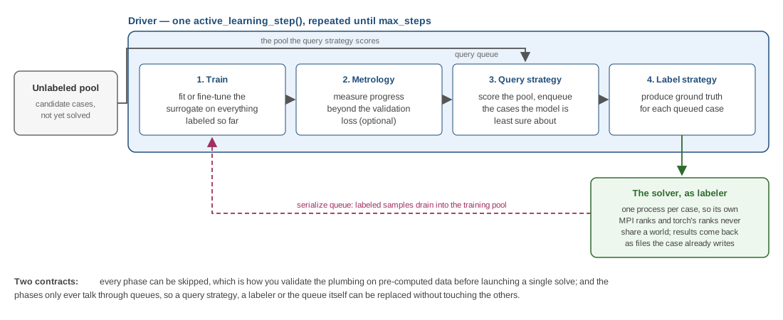
Figure 1: One step is train, measure, query, label. The solver is the labeler, and the queues between the phases are what make it pluggable.
One active_learning_step() runs the four phases in order; Driver.run() repeats it until max_steps. Any phase can be switched off (skip_training, skip_metrology, skip_labeling), which is how you validate the plumbing with pre-computed data before a single solve is launched.
Phases talk through queues. The query strategy puts samples on a queue; the label strategy takes them off, labels them, and puts the results on a second queue; the driver drains that into the training pool. The queue type is a protocol too (AbstractQueue), so a multiprocessing or distributed queue drops in.
Protocols, not base classes
Every pluggable piece is a typing.Protocol: as long as an object has the right methods and attributes at run time, it fits — no inheritance required. That is what lets a label strategy be defined lazily against physicsnemo without importing it at module scope, which matters when physicsnemo is an optional dependency.
| Protocol | You provide | Called |
|---|---|---|
QueryStrategy | max_samples, sample(query_queue) — reads driver.unlabeled_pool, scores candidates, enqueues the chosen ones | once per step, phase 3 |
LabelStrategy | label(queue_to_label, serialize_queue), plus __is_external_process__ (a solver is involved) and __provides_fields__ (the field names it adds) | once per step, phase 4 |
MetrologyStrategy | any measurement of progress beyond the validation loss | once per step, phase 2, optional |
TrainingProtocol, ValidationProtocol, InferenceProtocol | one training step, one validation step, one inference step | inside the TrainingLoop |
TrainingLoop | the epoch loop; DefaultTrainingLoop is the ready-made one | phase 1 |
All of them share ActiveLearningProtocol: a __protocol_name__, an attach(driver) that gives the strategy the driver's scope (driver.learner, the pools, the configs, the checkpoint directories), a configured logger, and checkpoint_dir/strategy_dir for anything it wants to persist.
The Driver and its configs
Driver is the orchestrator. It is configured by dataclasses:
| Config | Holds |
|---|---|
DriverConfig | infrastructure — batch size, logging, distributed settings, max_steps, checkpoint_interval, the skip flags |
StrategiesConfig | the strategy instances: query, label, metrology, training loop |
TrainingConfig | the training components — datapools, optimizer, scheduler, epochs per step |
OptimizerConfig | the optimizer's own parameters |
It wraps the learner in DistributedDataParallel when ranks exist, checkpoints configurations, weights, optimizer state and queue contents at checkpoint_interval, injects the step index and phase into every log line, and resumes from load_checkpoint(checkpoint_dir). Artifacts of a run: .mdlus checkpoints per step, driver_log.json with the timeline, and whatever the metrology strategy writes.
One contract that is easy to miss: TrainingConfig needs a train_datapool even when training is skipped, because labeled samples are drained into it after phase 4.
Query strategies worth knowing
| Strategy | Signal | Cost | When |
|---|---|---|---|
| random | none | none | the baseline everything must beat; competitive early on |
| ensemble disagreement | variance across K trained models | K trainings | when you already train an ensemble for error bars |
| predictive entropy | the model's own output distribution | one pass | classifiers, or a diffusion ensemble's spread |
| physics residual | how badly the prediction violates the governing equations | one residual assembly per candidate | when a solver exists — this is the one only a solver-backed setup can offer |
| hybrid | e.g. 60 % uncertainty, 40 % random | guards against the training set collapsing onto one region |
An honest finding worth repeating: on smooth one- and two-parameter families, two or three solves saturate the surrogate and active learning is indistinguishable from random. The machinery pays off when the family is rough or high-dimensional, not before — so measure against the random baseline before believing a query strategy is earning its cost.
Where the solver sits
The solver is the label strategy. Each queried sample becomes a real solve through an execution backend, and the choice of backend is the one design decision that matters:
- an in-process backend runs the solve in the current interpreter — fine for small problems and notebooks;
- a subprocess backend launches one solver process per case, which keeps the solver's own MPI ranks and torch's distributed ranks in separate operating-system processes, fans out over a job limit, and becomes an HPC job submission with an
srunorsbatch --waitprefix. Results come back as whatever files the case was configured to write.
The second is the right default for anything real, and the reason is not performance: a solver and a training process that both think they own the MPI world will deadlock or, worse, silently disagree about rank identity.
In meshio++
meshio++ sits on both sides of the loop without implementing any of it.
On the label side, a solve's output becomes training data through the ordinary path: write_dataset or a DatasetManifest entry, and dataset_add over MCP so an agent-driven loop can register the new case without a Python import. Because the manifest is a hand-editable JSON that tools and people both write, a labeling step appending to it is a two-line operation rather than a bespoke serialization format.
On the query side, estimate_error is the closest thing to the physics-residual strategy that works with no solver in the loop: a recovered-gradient indicator per cell, with Dorfler bulk-chunk marking. It ranks where within one mesh the field is untrustworthy, not which case to solve next — the two are different questions, and only the second is what a query strategy answers.
The loop itself is not built and is not planned. Its natural home is the process that owns the solver, and meshio++ owns neither the solver nor the training loop's outer schedule.