Field derivatives — gradient, divergence, curl

gradient(mesh, array, operator=…, method=…, location=…) differentiates a point_data field over the mesh: its gradient, divergence or curl. It is a mesh operation, not a file format, uses only standard C++/numpy, and runs under every mesh backend.

meshio++ could already transform, transfer (interpolate), summarize (data operations) and contour (isosurface) a field. This is what lets it differentiate one, which is the missing input for the two workflows at the bottom of this page: contouring a derived quantity, and driving the selective refine from a gradient-based error indicator.

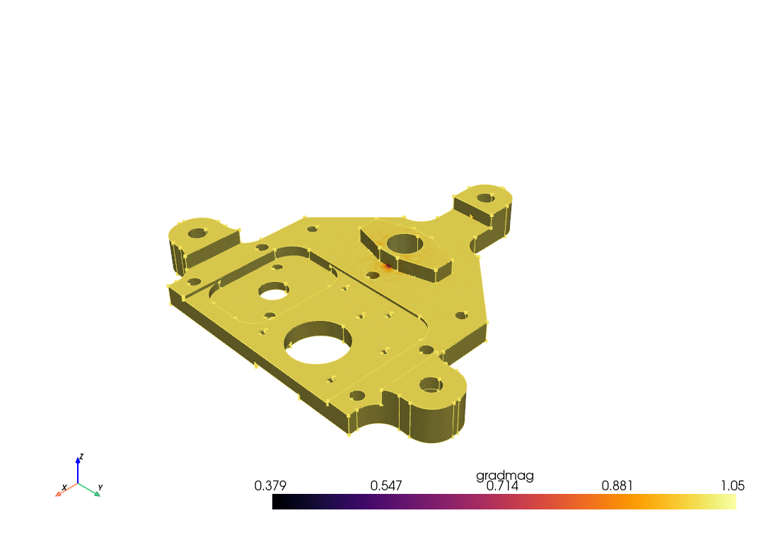
import meshioplusplus as mp

mesh = mp.read("solution.vtu")

g = mp.gradient(mesh, "T")                          # cell_data["T:gradient"], (n, 3)
g = mp.gradient(mesh, "T", location="point")        # point_data instead
g = mp.gradient(mesh, "u", operator="curl")         # vorticity, (n, 3)
d = mp.gradient(mesh, "u", operator="divergence")   # (n,)

out, report = mp.gradient(mesh, "T", return_report=True)
report["num_skipped"]   # cells that could not be differentiated (NaN rows)
report["num_fallback"]  # least-squares cells that fell back to Green-Gauss

Where it lives, and why

The five data operations are defined by never touching geometry. This one consumes and produces data arrays but reads geometry and topology — face areas, cell volumes, cell-to-cell adjacency — so it lives in the mesh-operations layer (operations/gradient.hpp) alongside smooth and isosurface, not in the data_* family.

It is still reachable as meshioplusplus data gradient in both CLIs, because that is where a user looks for it. That is the one deliberate inconsistency in the data group, and it is noted in its help text.

The two methods

Method	What it does	Exact for a linear field
green-gauss (default)	Divergence theorem over the cell's own faces (3-D) or corner ring (2-D). Uses only the cell itself.	Any 3-D cell; any planar 2-D cell
least-squares	Linear fit over the cells sharing at least one node.	3-D meshes; planar 2-D meshes

Green-Gauss is the right default: it is local (no neighbour stencil, so no sensitivity to how the mesh is connected), cheap, and exact on a wider class of cells. Reach for least-squares when the field is under-resolved and you want the smoothing a wider stencil gives, or on a mesh of very high aspect ratio, where the neighbour fit is better conditioned than a single cell's faces.

Green-Gauss

For each face, the corners are fanned into triangles about the face's arithmetic corner average, and each sub-triangle contributes A_j · f(centroid_j):

c   = mean(face corner coords)        fc  = mean(face corner values)
A_j = ½ (p_i − c) × (p_{i+1} − c)
f_j = (fc + f(p_i) + f(p_{i+1})) / 3
grad f = (Σ f_j A_j) / V,   V = ⅓ Σ (centroid_j · A_j)

This is exact for a linear field on any cell — planar faces or not. Two faces sharing an edge contribute oppositely-wound triangles on that edge, so the fan surface is closed, and ∮ f n dA = V ∇f is a purely algebraic identity on a closed oriented piecewise-linear surface. V is the exact signed volume of that same fan surface, so numerator and denominator flip together and an inverted cell yields the same gradient as its positively-wound twin.

Why the fan, and why that apex

The corner-average apex is forced, not convenient: the quadrature needs f at the apex, and for linear f the corner average is the only point whose value is known exactly without shape functions (mean(f(pᵢ)) = f(mean(pᵢ))).

Skipping the fan and using the plain corner-average face value is wrong by 12.5 % on the trapezoid (0,0),(4,0),(2,1),(0,1) under f = y. A cube cannot detect this — for a parallelogram the corner average is the area centroid — which is why the test fixtures are a frustum and a warped hex.

On a 2-D cell the same theorem runs over the corner ring with the in-plane outward normal t × N, where N is the cell's own Newell normal. That is exact on a planar cell, invariant under both reversal and cyclic rotation of the ring, and first-order on a warped quad in 3-D, which has no well-defined area or normal to begin with.

Least-squares

f(x) ≈ f_c + g · (x − x_c) is fitted over the cells sharing at least one node, with x_c and f_c the cell's arithmetic corner averages — so (x_c, f_c) lies exactly on a linear field and the fit is exact for one under any positive weights. Weights are 1/|d|², which makes the normal matrix Σ d̂ d̂ᵀ: dimensionless, immune to mesh grading, and scale-invariant.

The neighbour definition (node-sharing, ascending global cell index, de-duplicated) is shared with partition's ghost layers via detail/cell_adjacency.hpp, so the two cannot disagree.

On a 2-D mesh the offsets are projected into the cell's plane, so exactness holds on a planar mesh and degrades to first-order on a curved surface, where the projection discards a real part of the offset.

A degenerate neighbourhood — an isolated cell, a collinear strip — falls back to Green-Gauss for that cell and is counted in num_fallback. It is never silently wrong and never NaN when a usable answer exists.

Shapes and naming

An nc-component input yields 3 · nc gradient components, flat and row-major as [component i][derivative j] at index i * 3 + j:

Input	Operator	Output	Layout
scalar (n,)	gradient	(n, 3)	∂f/∂x, ∂f/∂y, ∂f/∂z
vector (n, 3)	gradient	(n, 9)	∂u/∂x … ∂u/∂z, ∂v/∂x … , ∂w/∂x …
vector (n, 3)	divergence	(n,)	∂u/∂x + ∂v/∂y + ∂w/∂z
vector (n, 3)	curl	(n, 3)	∂w/∂y − ∂v/∂z, ∂u/∂z − ∂w/∂x, ∂v/∂x − ∂u/∂y

component=i selects one component of a multi-component input and yields 3 (gradient only — setting it with divergence or curl is an error, not a silently ignored argument).

Divergence and curl need 2 or 3 components. A 2-component field reads as (u, v, 0), the same padding convention 2-D point coordinates already use.

Output is always Float64 — a derivative is not an integer — and named <input>:gradient / :divergence / :curl unless output= overrides it. That is name:suffix, deliberately not the repo's usual prefix:name (iso:value, partition:part), so that everything derived from one field sorts next to it.

Boundaries, skipped cells and NaN

Boundary cells need no special case under Green-Gauss: the boundary face contributes with its own nodal mean, exactly like an interior one. Under least-squares a boundary cell simply has a smaller stencil, which is only a problem if it becomes rank-deficient — and then it falls back and is counted.

Cells that cannot be differentiated yield a NaN row and increment num_skipped, never an approximation:

• blocks below the mesh's own max topological dimension (a boundary triangle block on a tet mesh);
• ragged polygon and polyhedron blocks;
• 3-D types with no face table — the 3-D Lagrange family (hexahedron64 and up). 2-D Lagrange types are supported, since the corner ring is all that is needed;
• cells whose volume or area is degenerate relative to their own size (never an absolute epsilon), which would otherwise divide by ~0.

Higher-order cells are differentiated on their corner geometry — tetra10 is treated as its linear parent, and the mid-side values do not contribute. This is the same corner-only convention compute_quality and cell_measure use.

Non-finite input

Unlike every data_* operation there is no nan_policy here. Green-Gauss has no reduction to exclude a value from, so a single non-finite corner poisons its whole cell. Clean the field first (data clamp, data drop) if that matters.

Determinism

Output is byte-identical across the three mesh backends, across thread counts, and across the C++-core / numpy-fallback boundary (pinned by tests/python/test_gradient.py::test_cpp_matches_python). Per-cell work is independent and runs in parallel, but every accumulation inside a cell runs in a fixed order — faces in table order, fan triangles in ring order, neighbours in ascending global cell index — because floating-point addition is not associative. Point-located output rides cell_data_to_point_data, whose scatter is already deliberately serial.

One consequence worth stating: point-located values of a linear field are exact to within rounding, not bit-exact, because summing n copies of g and dividing by n is not exactly g in IEEE arithmetic.

Coordinates and values are recentred on the cell's corner average before any arithmetic. V = ⅓ Σ xⱼ · Aⱼ only telescopes because Σ Aⱼ = 0; on a mesh at x ~ 1e8 the raw form loses eight digits to cancellation and then divides by the result. Recentring changes nothing mathematically and removes the cancellation.

Worked compositions

These are the two reasons this operation exists.

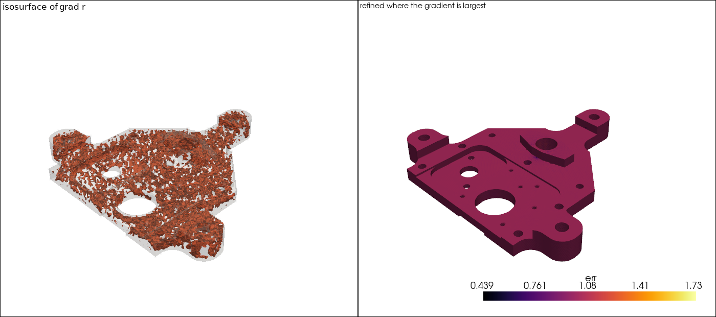
Contour a derived quantity

isosurface needs a point_data scalar. A gradient magnitude is exactly that, once you take the norm:

import numpy as np
import meshioplusplus as mp

mesh = mp.read("solution.vtu")
g = mp.gradient(mesh, "T", location="point")
grad = np.asarray(g.point_data["T:gradient"])
g.point_data["gradT"] = np.sqrt((grad**2).sum(axis=1))

shells = mp.isosurface(g, "gradT", [2.0, 5.0])   # where T changes fastest
mp.write("thermal_shells.vtu", shells)

The same thing from the shell, in three verbs:

meshioplusplus data gradient solution.vtu g.vtu --array T --location point
meshioplusplus data calc g.vtu m.vtu --point 'gradT = norm(`T:gradient`)'
meshioplusplus isosurface m.vtu shells.vtu --array gradT --values=2.0,5.0

For a velocity field the same shape gives vorticity magnitude — swap --op gradient for --op curl.

Drive adaptive refinement

refine's --where selector takes any scalar cell_data, and a gradient magnitude is the classic error indicator: refine where the solution changes fastest.

g = mp.gradient(mesh, "T")                       # cell-located, the default
grad = [np.asarray(a) for a in g.cell_data["T:gradient"]]
g.cell_data["err"] = [np.sqrt((a**2).sum(axis=1)) for a in grad]

adapted = mp.refine(g, where="err > 3.0")        # 2:1-balanced by default

meshioplusplus data gradient solution.vtu g.vtu --array T
meshioplusplus data calc g.vtu m.vtu --cell 'err = norm(`T:gradient`)'
meshioplusplus refine m.vtu adapted.vtu --where "err > 3.0" --closure redgreen

Keep the gradient cell-located here: refine --where reads cell_data, so a point-located result would need averaging back onto the cells first.

CLI

meshioplusplus data gradient IN OUT --array NAME \
    [--op gradient|divergence|curl] \
    [--method green-gauss|least-squares] \
    [--location cell|point] \
    [--output NAME] [--component I] [--overwrite] [--quiet]

Both CLIs produce byte-identical files. See the CLI reference.

Other languages

int64_t skipped = 0, fallback = 0;
mio_mesh* g = mio_gradient(mesh, "T", "gradient", "green-gauss", "cell",
                           NULL, -1, 0, &skipped, &fallback);

type(mio_mesh) :: g
integer(int64) :: nskip, nfall
g = m%gradient('T', method='least-squares', num_skipped=nskip, num_fallback=nfall)

g = gradient(mesh, "T"; operator=:curl, location=:point)
g.mesh, g.num_skipped, g.num_fallback

g <- mio_gradient(mesh, "T", op = "curl", location = "point")
g$mesh; g$num_skipped

const g = await m.gradient(mesh, 'T', 'gradient', 'green-gauss', 'cell');
g.mesh.cell_data_components['T:gradient'];  // 3 — the shape travels with it

Two conventions differ across these surfaces and are worth pinning down:

• component is negative for every component here — deliberately the opposite of isosurface, where negative means the row magnitude. Both are documented at each binding.
• On the flat ABIs (C, Fortran, Julia, R, WASM) the counters are out-parameters or fields of a returned record, never an opaque handle: there are no index maps to hand back, so smooth's shape is the right one.

The browser viewer exposes this as the Derivative chip; because it changes no geometry, the result simply appears in the colour-by menu.