Isosurfaces / contours

meshioplusplus.isosurface(mesh, array, isovalues) computes the level set of a scalar field — the locus where a point_data array equals a given isovalue — as a mesh one topological dimension below the cut cells. It is a mesh operation, not a file format, uses only standard C++/numpy, and runs under every mesh backend.

• a 3D volume mesh yields a surface mesh (triangle/quad faces);
• a 2D surface mesh yields a line mesh (contour segments).

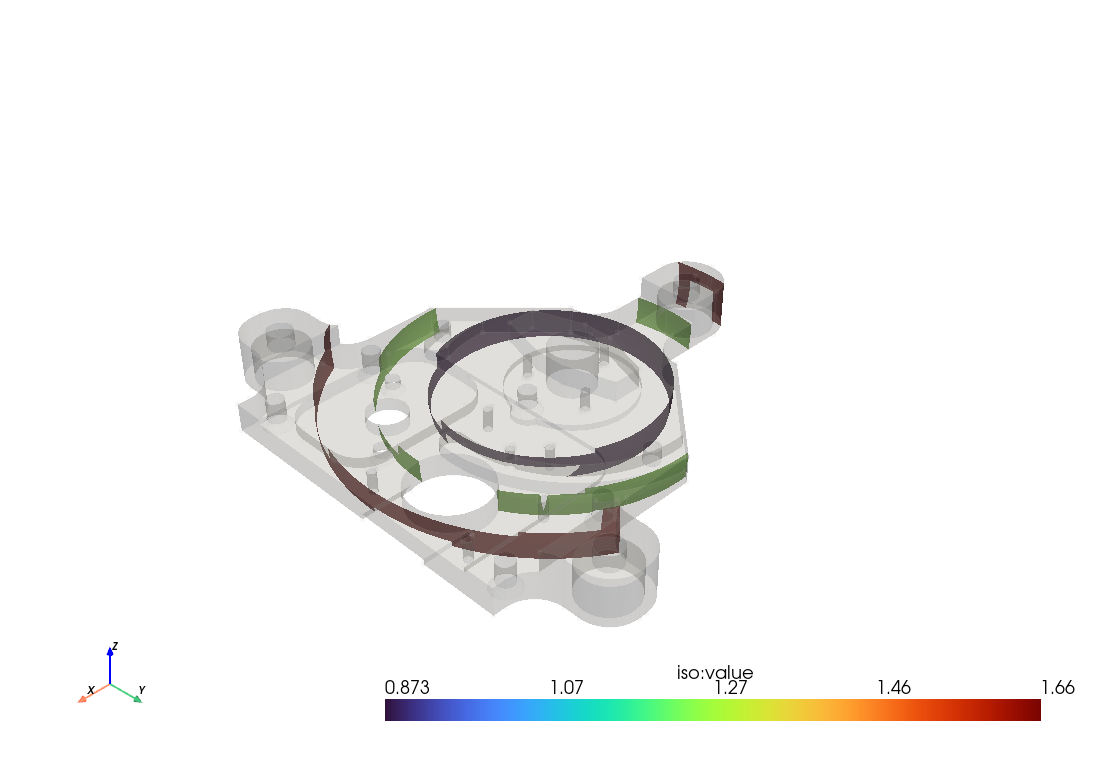
This is the data-driven sibling of slice: slice cuts where dot(x − origin, normal) = 0, isosurface where f(x) − isovalue = 0. They share one cutter, so everything below about watertightness, winding, degeneracy and determinism is literally the same code.

import meshioplusplus

vol = meshioplusplus.read("part.vtu")            # carrying point_data["T"]

# one level set
shell = meshioplusplus.isosurface(vol, "T", 350.0)

# several at once -- they all land in one mesh, tagged per cell
shells = meshioplusplus.isosurface(vol, "T", [300.0, 350.0, 400.0])

meshioplusplus.write("shells.vtu", shells)

The result is a brand-new mesh whose points are all cut points, so point_sets/cell_sets, mesh.info and gmsh_periodic are not carried; each contour cell inherits its parent cell's cell_data, and interpolated point_data is promoted to Float64.

The field must be point_data

cell_data is piecewise constant: it has one value per cell, so there is no crossing to locate inside a cell and no level set to draw. Naming a cell_data array raises by name, pointing at the conversion that fixes it:

# T lives on the cells -- move it to the points first
vol = meshioplusplus.cell_data_to_point_data(vol, ["T"])
shell = meshioplusplus.isosurface(vol, "T", 350.0)

meshioplusplus data to-point part.vtu nodal.vtu --cell T
meshioplusplus isosurface nodal.vtu shell.vtu --array T --values 350

A multi-component array reduces to a single component with component=, or to the row magnitude when that is left unset:

meshioplusplus.isosurface(vol, "velocity", 1.0, component=2)  # w = 1
meshioplusplus.isosurface(vol, "velocity", 1.0)               # |v| = 1

Several isovalues, one mesh

The isovalues are sorted ascending and exact duplicates are dropped, then cut in that order and concatenated with the section blocks merged by cell type — so a single-isovalue call has exactly slice's block structure. Every contour cell is tagged twice:

cell_data	dtype	meaning
iso:value	Float64	the isovalue this cell belongs to
iso:index	Int64	its ordinal in the ascending isovalue list

Both exist because they answer different questions. iso:value is the physical level you colour or label by; iso:index is the integer that split's tag criterion needs — that criterion only accepts integer arrays, so splitting into one file per contour goes through the ordinal (the CLI/Python spelling is region, which falls back to the named tag when the mesh carries no cell_sets, as a contour never does):

per_contour = meshioplusplus.split(shells, by="region", tag="iso:index")

meshioplusplus isosurface part.vtu shells.vtu --array T --values 300,350,400
meshioplusplus split shells.vtu 'contour_{key}.vtu' --by region --tag iso:index

An isovalue outside the field's range yields an empty contour for that value rather than an error; if every value is outside, the result is an empty mesh.

The contoured field is exactly the isovalue

Every point_data array is interpolated at the crossing parameter t = d_lo / (d_lo − d_hi), which is exact for a linear field. The contoured array's own value would only reach the isovalue to within round-off, so it is written exactly instead — iso.point_data["T"] == 350.0 holds bit for bit, not merely to a tolerance.

The one exception is a multi-component array reduced by magnitude: |lerp(v)| ≠ lerp(|v|) mathematically, not merely in floating point, so there is no exact value to write and that case stays approximate. Selecting a component restores exactness for that component.

How it works — marching tetrahedra

The input is first simplexified with convert_cells (every 3D cell becomes a tetrahedron, every 2D cell a triangle), so each cell's contour is a well-defined convex primitive — no angular point-sorting and no non-convex-hex ambiguity. Per simplex the level set crosses 0, 3 or 4 edges of a tetra (a triangle or quad) or 0 or 2 edges of a triangle (a line), from a fixed case table keyed by the vertices' above/below-isovalue pattern.

The honest consequence: a hexahedron or wedge contour is the union of its simplices' contours — correctly located and shaped, just triangulated rather than returned as a single polygon. The field is resolved against the simplexified mesh, so a higher-order input contours the linearized field.

Degeneracy rule — plateaus

A node whose value is exactly the isovalue (d_i == 0) is classified on the positive side (d_i >= 0). This one rule makes the sign mask total, which is what keeps the contour well-defined at the awkward cases:

• a plateau region sitting exactly at the isovalue emits its boundary once, from one of the two incident cells — never doubled;
• any contour primitive whose crossings collapse to a point or a line (area or length below a bbox-relative tolerance) is dropped, so there are no zero-area/zero-length contour cells.

Watertight contours

A crossing point on an edge shared by two simplices is emitted as a single output node: cut points are keyed by the sorted pair of simplexified-node ids and deduped, so the contour is watertight. The documented exception is a plateau configuration (the level set passing exactly through mesh vertices/edges), where coincident-but-distinct nodes can remain — the contour is still geometrically correct, just not vertex-minimal there.

Winding

Every contour face is wound so that its Newell normal points toward increasing field — a globally consistent orientation (the level set of a temperature field faces the hotter side), pinned by a Newell-normal invariant test (tests/cpp/test_isosurface.cpp). The per-simplex reference direction is the centroid of the corners at or above the isovalue minus the centroid of those below, which needs no gradient solve and reproduces exactly in numpy.

Provenance

With record_parent_ids=True, an Int64 iso:parent_cell cell_data array records, per contour cell, the global (block-major) index of the input cell it was cut from — mirroring slice:parent_cell and surface:parent_cell. The parent's cell_data row is replicated onto each contour cell regardless of this flag.

Determinism

Output is byte-identical across the three mesh backends, across thread counts, and across the C++-core / numpy-fallback boundary (pinned by tests/python/test_isosurface.py::test_cpp_matches_python): the field-evaluation and coordinate/point_data passes are parallel, but the cut-and-dedup sweep that hands out node ids is serial over a fixed (block, cell, ring-edge) traversal, the crossing t is computed from the sorted endpoint pair so both sides of a shared edge agree bit-for-bit, and the contours are concatenated in ascending isovalue order.

CLI

meshioplusplus isosurface IN OUT --array T --values 350
meshioplusplus isosurface part.vtu shells.vtu --array T --values 300,350,400
meshioplusplus isosurface part.vtu shell.vtu --array v --values=-1.5 --component 2

Negative isovalues use the --values=… form (a bare --values -1.5 would be read as a new option). Available in both the Python CLI and the native meshioplusplus binary — see the CLI reference.

Other languages

The operation is exposed on every binding surface:

/* C API */
double isovalues[2] = {300.0, 350.0};
mio_mesh* shells = mio_isosurface(mesh, "T", isovalues, 2,
                                  /*component=*/-1, /*record_parent_ids=*/1);

! Fortran: type-bound procedure (like m%slice / m%crop_plane)
shells = mesh%isosurface('T', [300.d0, 350.d0], record_parent_ids=.true.)

// WASM
const shells = m.isosurface(mesh, 'T', [300, 350], -1, true);

component crosses the flat ABIs as an int with negative meaning magnitude (None in Python). As everywhere on the flat bindings, point_sets/cell_sets never cross — and here they are not carried at all, since the contour is entirely new topology. The browser viewer's isosurface chip runs this operation.