Second derivatives — the Hessian

hessian(mesh, array, method=…, location=…) computes the second derivative (Hessian matrix) of a scalar point_data field — gradient's companion one order further: gradient differentiates a field once, this differentiates it twice. It is a mesh operation, not a file format, uses only standard C++/numpy, and runs under every mesh backend.

For curvature-driven adaptive refinement (the motivation this closes), a first-derivative magnitude is a weak proxy: it is large on a steep-but-straight ramp and misses a sharp bend in an otherwise-flat field. A Hessian-based indicator is the standard fix.

import meshioplusplus as mp

mesh = mp.read("solution.vtu")

h = mp.hessian(mesh, "T")                          # cell_data["T:hessian"], (n, 9)
h = mp.hessian(mesh, "T", location="point")        # point_data instead
h = mp.hessian(mesh, "T", method="least-squares")  # forwarded to both internal passes

out, report = mp.hessian(mesh, "T", return_report=True)
report["num_skipped"]   # cells that could not be evaluated (NaN rows)
report["num_fallback"]  # least-squares cells that fell back, in either pass

Composition, not a new numerical kernel

hessian is built entirely out of two calls to gradient — exactly the precedent estimate_error already sets:

1. gradient(array, location="point") gives the field's gradient as a genuine point_data array, (n, 3).
2. gradient again on that array, with the default "gradient" operator — which is generic over its input's own component count — differentiates a 3-component field and so produces (n, 9): the flattened row-major 3×3 Hessian, H[i][j] = ∂²f/∂xᵢ∂xⱼ at index i*3+j.

The first internal call must use location="point", regardless of what the caller asked for: the second call's point_data-only validation would otherwise reject a cell_data intermediate. method simply forwards to both internal gradient calls, so "least-squares" is available for free, exactly as it already is for gradient itself — no new differentiation math is written for hessian at all.

Where it lives, and why

Same reasoning as gradient/estimate_error/data_integrate: the five data operations are defined by never touching geometry. hessian reads geometry indirectly (through the two gradient calls it composes), so it lives in the mesh-operations layer, not the data_* family. It is still reachable as meshioplusplus data hessian in both CLIs, because that is where a user looks for it.

Exactness — stated honestly, not oversold

The rigorous, mesh-shape-independent guarantee: a field that is at most linear has an exactly zero Hessian everywhere. Its gradient is a constant, and Green-Gauss of a spatially constant field is trivially exact — ∮ f̄ n dA = f̄ ∮ n dA = 0 over any closed surface. This is the same class of guarantee gradient's own identity test (CurlOfAGradientAndDivergenceOfACurlVanish) relies on, for the identical reason.

For a genuinely quadratic field, each Green-Gauss pass alone would be exact (the gradient of a quadratic field is linear), but the mandatory intermediate step — cell_data_to_point_data(weight="uniform"), a plain arithmetic mean of incident-cell values — is only exact for a field that is constant over the averaged neighbourhood. For a genuinely-varying linear field (i.e. the gradient of a true quadratic), averaging several cells' individually-exact-but-different local values reproduces the true nodal value only when those cells are symmetric about the shared node.

Measured, not merely argued: on a regular axis-aligned hex grid, every interior node's 8-cell neighbourhood is exactly that symmetric, and the composed Hessian comes back exact to machine precision there. The same mesh's own boundary cells (a one-sided, asymmetric neighbourhood) show real, bounded error — tests/cpp/test_hessian.cpp's QuadraticFieldOnAStructuredGridIsExactAwayFromTheBoundary and ...HasBoundedBoundaryError pin both halves on the identical mesh.

So the composed Hessian is exact away from a mesh's own boundary on a structured/symmetric mesh, and a good, standard, but genuinely approximate curvature estimate on an irregular mesh — the same honesty gradient's own doc uses ("first-order on a warped quad in 3-D") rather than a blanket exactness claim. A full quadratic-least-squares Hessian recovery would restore mesh-shape independence but is a substantially larger undertaking and out of scope here.

Scope: scalar fields only

The input must have exactly one component. A vector field's Hessian is a separate quantity per component ((n, 3) in → nine numbers per component out) — a real but different need, refused by name rather than guessed at:

mp.hessian(mesh, "velocity")
# ValueError: 'velocity' has 3 components; hessian currently supports
# scalar fields only -- call it once per component of a vector field

Shapes and naming

A scalar input yields (n, 9), row-major flattened H[i][j] at index i*3+j:

∂²f/∂x²    ∂²f/∂x∂y   ∂²f/∂x∂z
∂²f/∂y∂x   ∂²f/∂y²    ∂²f/∂y∂z
∂²f/∂z∂x   ∂²f/∂z∂y   ∂²f/∂z²

Output is always Float64, and named <input>:hessian unless output= overrides it — the direct extension of gradient's own <input>:gradient naming rule, so a caller already reading T:gradient knows how to read T:hessian.

Skipped cells and NaN

Cells that cannot be evaluated read NaN and increment num_skipped — the second internal gradient pass's own count, which structurally coincides with the first pass's own skip set (both run over the identical mesh topology): unsupported types, wrong topological dimension, ragged/polyhedron blocks, and a degenerate measure. There is no separate NanPolicy here, the same as gradient and data_info.

Worked composition: curvature-driven refinement

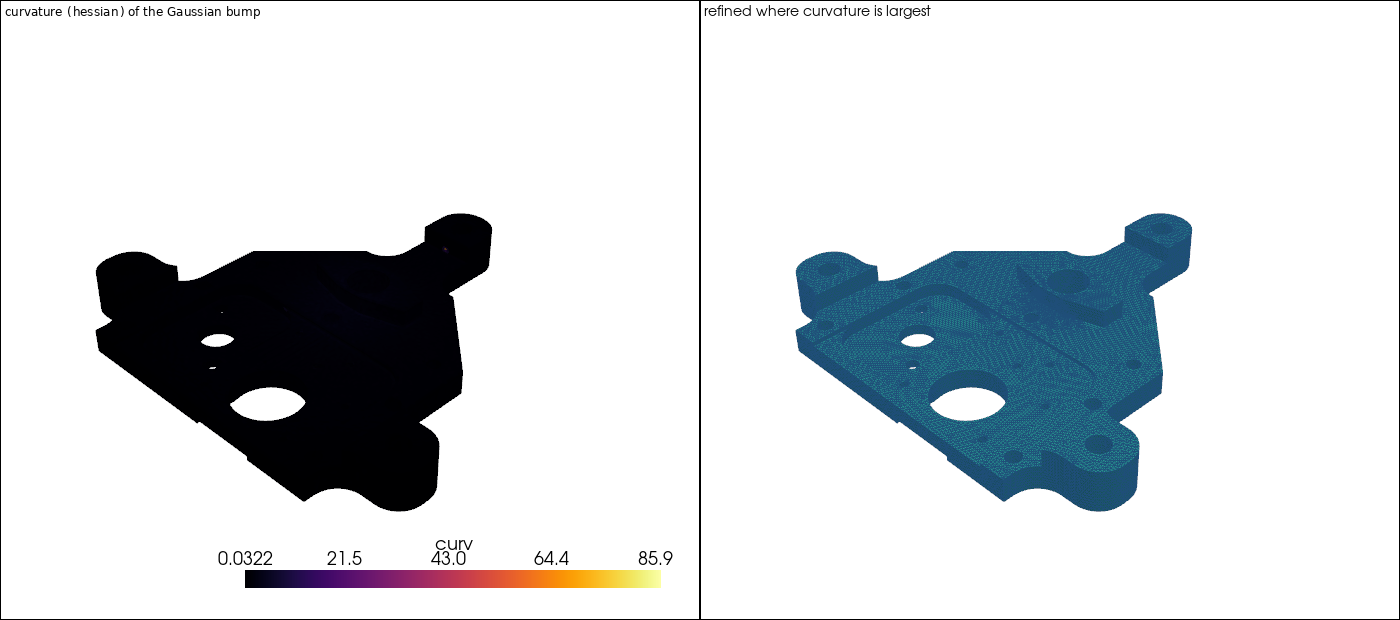
data_calc's norm(...) is a plain sum-of-squares-then-sqrt over however many components its argument has, so norm(hessian_array) on the 9-component output is exactly its Frobenius norm — a scalar curvature indicator with zero new code, ready for refine's --where selector. No bespoke marking pass is needed here, unlike estimate_error's ZZ-specific one: the composable pieces already exist and are more general.

import meshioplusplus as mp

mesh = mp.read("solution.vtu")
h = mp.hessian(mesh, "T")                                  # cell-located, the default
curv = mp.data_calc(h, "norm(`T:hessian`)", location="cell", output="curv")
adapted = mp.refine(curv, where="curv > 3.0")               # 2:1-balanced by default

The same thing from the shell, in three verbs:

meshioplusplus data hessian solution.vtu h.vtu --array T
meshioplusplus data calc h.vtu m.vtu --cell 'curv = norm(`T:hessian`)'
meshioplusplus refine m.vtu adapted.vtu --where "curv > 3.0" --closure redgreen

Note the --cell location: refine --where reads cell_data, so a point-located Hessian would need averaging back onto the cells first.

CLI

meshioplusplus data hessian IN OUT --array NAME \
    [--method green-gauss|least-squares] \
    [--location cell|point] \
    [--output NAME] [--overwrite] [--quiet]

Both CLIs produce byte-identical files. See the CLI reference.

Other languages

int64_t skipped = 0, fallback = 0;
mio_mesh* h = mio_hessian(mesh, "T", "green-gauss", "cell", NULL, 0, &skipped, &fallback);

type(mio_mesh) :: h
integer(int64) :: nskip, nfall
h = m%hessian('T', method='least-squares', num_skipped=nskip, num_fallback=nfall)

h = hessian(mesh, "T"; location=:point)
h.mesh, h.num_skipped, h.num_fallback

h <- mio_hessian(mesh, "T", location = "point")
h$mesh; h$num_skipped

const h = await m.hessian(mesh, 'T', 'green-gauss', 'cell');
h.mesh.cell_data_components['T:hessian'];  // 9 — the shape travels with it

Also reachable as a convertSurfaceOps/settings-pipeline step ({op: 'hessian', array, method, location, output} in WASM; {"Op": "Hessian", "Array": ..., "Method": ..., "Location": ..., "Output": ...} in a settings.json), exactly like gradient — a pure data step that changes no geometry, so the mesh passes straight through with one array attached.

The browser viewer has no dedicated Hessian chip; the array attaches like any other pipeline step's output and is available in the colour-by menu once the pipeline runs.