Training utilities and performance

physicsnemo.utils is the part of the library that is not about models at all: capturing a training step into a CUDA graph, mixed precision, profiling, logging, resumable checkpoints. physicsnemo.optim adds two optimizers. None of it is required — a plain torch loop works — which is why most loops start plain and grow into it.

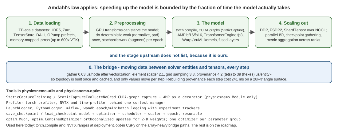
Figure 1: Where the time goes. Upstream lists four stages; a solver or mesh coupling adds a fifth.

How upstream thinks about performance

The performance guide opens with Amdahl's law: the gain from speeding up one part is bounded by the fraction of time that part takes. It then names four places time goes, and for scientific ML the surprise is how often the model is not the bottleneck:

1. Data loading. Datasets are measured in terabytes; single samples can be gigabytes. HDF5, Zarr and TensorStore readers, DALI, memory-mapped .pmsh meshes (upstream measured 20 to 135x faster loads than VTU and 2 to 7x smaller files), and the IOPump prefetcher exist for this stage.
2. Preprocessing. GPU-side transforms can starve the model. Deterministic work (normalization, padding) belongs in a one-off pass or in the exporter; stochastic work (augmentation) per epoch.
3. The model. torch.compile, CUDA graphs, mixed precision, TransformerEngine's fp8 attention (use_te), and specialized kernels in Warp and cuML.
4. Scaling out. Data or domain parallelism over NCCL, plus the unglamorous parts: parallel I/O, gathering checkpoints, aggregating metrics across ranks.

And a fifth stage whenever a mesh is involved: turning mesh entities into tensors. Nodal value gathering is cheap; building the topology — the edge graph, the tessellation, the provenance map — is not, and it is a hundred times more expensive per element. The rule that follows is the whole of it: topology once, values every step.

The tools

Tool	What it does	Notes
StaticCaptureTraining, StaticCaptureEvaluateNoGrad	decorators that capture a training (or evaluation) function into a CUDA graph after a warm-up, with AMP (amp_type float16 or bfloat16) and optional torch.compile	require a physicsnemo.Module; the model's ModelMetaData declares whether it supports CUDA graphs and AMP
Profiler	one context manager configuring the torch profiler, NVTX ranges and line profiling together	pairs with Nsight Systems
LaunchLogger, PythonLogger, RankZeroLoggingWrapper	epoch and mini-batch logging with mlflow and Weights and Biases back-ends, rank-0 only under distribution	the logging stack the upstream examples use
save_checkpoint, load_checkpoint, get_checkpoint_dir	a training checkpoint: models, optimizer, scheduler, grad scaler, epoch and metadata, local or remote (fsspec)	this is resumable training; the .mdlus written by Module.save is the deployable artifact, a different thing
physicsnemo.optim.Muon	orthogonalized (Newton-Schulz) updates for 2-D weight matrices, batched across same-shape parameters	a subclass of torch's Muon
physicsnemo.optim.CombinedOptimizer	different optimizers on different parameter groups	e.g. Muon on the matrices, Adam on everything else

The distinction in the middle of that table is the one people trip over: save_checkpoint writes a training checkpoint you can resume from, and Module.save writes a deployable one you can hand to somebody else. They are not substitutes and a pipeline usually wants both.

Three rules from profiling a mesh coupling

These came out of measuring a per-step coupling rather than reasoning about it, and they generalize:

1. Topology once, values every step. Extract connectivity in the setup phase and cache it; re-gather only field values per step. Rebuilding a graph every step cost 1073 ms on a 64k-node hexahedral mesh to keep 2.8 ms of node features.
2. The invalidation guard must match what the cache depends on. A cache holding a pure cell-to-entity map may key on the entity count; one holding simplex coordinates must compare coordinates. Copying a guard between caches produced one wrong answer and one needless rebuild.
3. Single-step tests cannot see per-step waste. Every one of these was invisible until a process ran for more than one step.

In meshio++

run_training is a plain torch loop, deliberately: epochs, an optimizer, a loss, per-epoch validation, best-and-last checkpoints, and a metrics.jsonl written incrementally so a dashboard can tail it. None of the upstream tooling above is wired in — no AMP, no CUDA-graph capture, no resumable optimizer state, no experiment tracker. That is a known gap kept separate from correctness work on purpose, and the honest statement is that for the mesh sizes this library is usually pointed at, stages 1 and 5 dominate stage 3 anyway.

Where meshio++ does invest is stage 1 and stage 5:

• Stage 1. write_dataset turns a whole campaign into one columnar dataset up front, so training reads Parquet or Zarr rather than re-parsing solver output every epoch. TimeSeries holds only a plan, so a thousand-solve dataset never has more than one mesh alive.
• Stage 5. Rule 1 above is structural here: graph_sample computes edge_index from the mesh's own topology, and a dataset that reuses one geometry across time steps pays for it once. to_dlpack and to_torch hand the arrays over with no copy where the buffer is already the right dtype, and pinned_reads() lets the reader allocate into pinned memory so the host-to-device transfer is a DMA rather than a staged copy.

The counterpart to Profiler here is much simpler and worth stating: every operation is deterministic and byte-identical across backends and thread counts, so a timing regression is a timing regression rather than a different answer.

Next: Distributed and scale.