Symbolic and physics

physicsnemo.sym

physicsnemo.sym lets you write a PDE in SymPy and get back something differentiable that scores how badly a network's output violates it.

• sym.eq.pde — the PDE base class you subclass to declare equations symbolically;
• sym.eq.phy_informer.PhysicsInformer — evaluates those equations on a network's output, producing per-point residuals you can add to a loss;
• sym.eq.gradients — the derivative machinery underneath, with several backends: autodiff at point coordinates, least squares on a mesh or graph, finite differences or spectral differentiation on a grid.

It ships bundled with physicsnemo 2.2 — no separate physicsnemo-sym install. Only SymPy itself is an extra.

physicsnemo.nn.functional.derivatives is the lower-level route to the same operators when you do not want SymPy at all.

Three things called "residual"

This is the distinction that matters most, and getting it wrong wastes weeks.

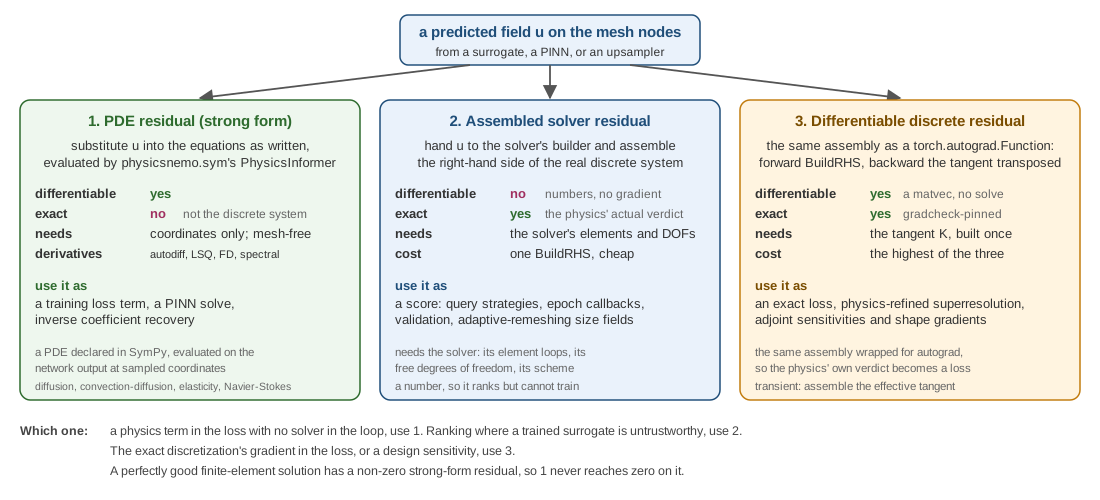
Figure 1: The three residuals, what each is exact or differentiable about, and what to use it for.

1. The PDE residual (approximate, differentiable)

Substitute the network's output into the strong form of the PDE and see what is left over. PhysicsInformer does this.

• Differentiable, so it can be a training loss.
• Mesh-free — it needs coordinates, not a discretization.
• It measures violation of the PDE, not of the discrete system a solver actually solves. A perfectly good finite-element solution has a non-zero strong-form residual pointwise.

2. The assembled solver residual (exact, not differentiable)

Hand the predicted field to the solver's own builder and assemble the real residual of the real discrete system.

• Exact — it is the physics' actual verdict on the prediction.
• Not differentiable: it is a number, not a gradient.
• Cheap enough to run often.

Use it as a score: active-learning query strategies ranking where the surrogate is weakest, epoch callbacks, validation.

3. The differentiable discrete residual (exact and differentiable)

The same assembly, wrapped as a torch.autograd.Function: forward assembles the right-hand side, backward applies the consistent tangent's transpose — a matrix-vector product, not a solve.

• Exact and gradient-carrying, so the physics' own verdict becomes a loss.
• The most expensive of the three.
• Only available where a solver exposes both an assembly routine and its tangent.

Which to use

You want	Use
A physics term in the loss, no solver in the loop	1
To rank where a trained surrogate is untrustworthy	2
The exact discretization's gradient in the loss	3

Sensitivities

The neighbouring question is "how does my objective change if I move something", and it has the same three-tier structure. A cheap surrogate dJ/dx comes free by autograd through any point-cloud interface. Exact adjoint parameter sensitivities need one solve of the transposed system for all parameters at once. A discretely exact dJ/dX at every node can be had from a single pass over the mesh, because moving a node perturbs only its adjacent entities — re-evaluating just those local right-hand sides replaces a per-parameter path's global assemblies with a cost linear in the mesh, and independent of the number of design parameters.

All of that lives on the solver side of the boundary. What a mesh library contributes is the geometry the sensitivity is taken with respect to, and the deformers that turn a handful of control parameters into a moved mesh.

In meshio++

Route 1 is the only one reachable without a solver, and meshio++ supplies its ingredients rather than the loss itself:

• gradient computes first derivatives (Green-Gauss or least squares) of any point_data field on any cell type, and hessian second derivatives, both exact for a field of the corresponding order. They are not differentiable — they run in the C++ core, not in an autograd graph — so they are the right tool for building features and for checking a physics term, not for being one.
• data_integrate gives the cell-measure-weighted totals a conservation check needs.
• estimate_error turns a recovered-gradient discrepancy into a per-cell indicator, which is the natural "where is this field untrustworthy" score when no solver is available to assemble a real residual — and it feeds refine's --where selector directly, closing an adaptive loop with no model in it at all.

Routes 2 and 3 need a live solver: an assembly routine, and for route 3 its tangent. That is deliberately outside this library's scope — meshio++ has no notion of a discrete system — and it is the clearest example of what a solver coupling adds over a mesh library. conservative_interpolate is the closest thing here: it preserves an integral exactly across two different discretizations, which is the property route 2 exists to check.

Next: Diffusion and deployment.