Scientific plots and FEM postprocessing

The Plots pane is a read-only analysis workspace inside the mesh editor, for point histories, SubModelPart quantities and spatial profiles. A standalone Scientific Plot Builder also handles CSV/TSV without a mesh. Both use the same host-side extraction and numerical calculations as MCP, rather than sampling the rendered viewport. You do not need a plotting script. These are delivered increments of roadmap item 19; the remaining acceptance work is listed below.

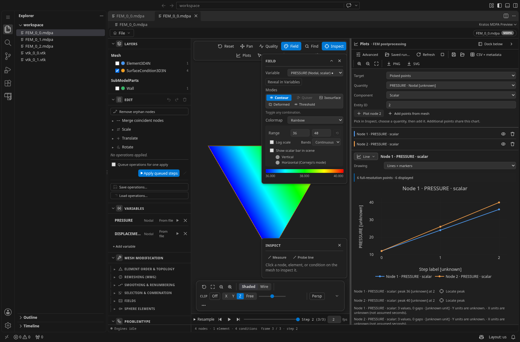
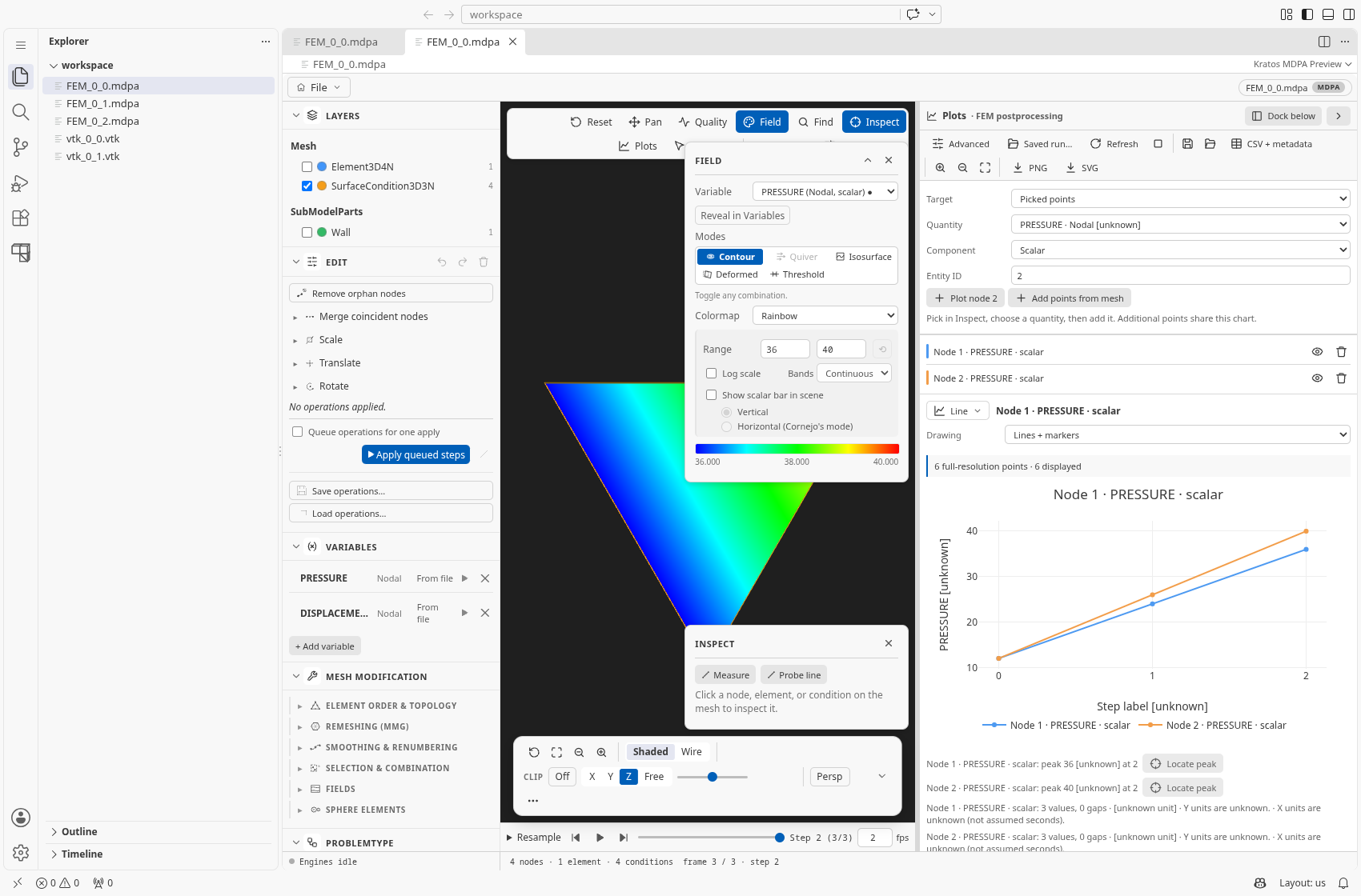
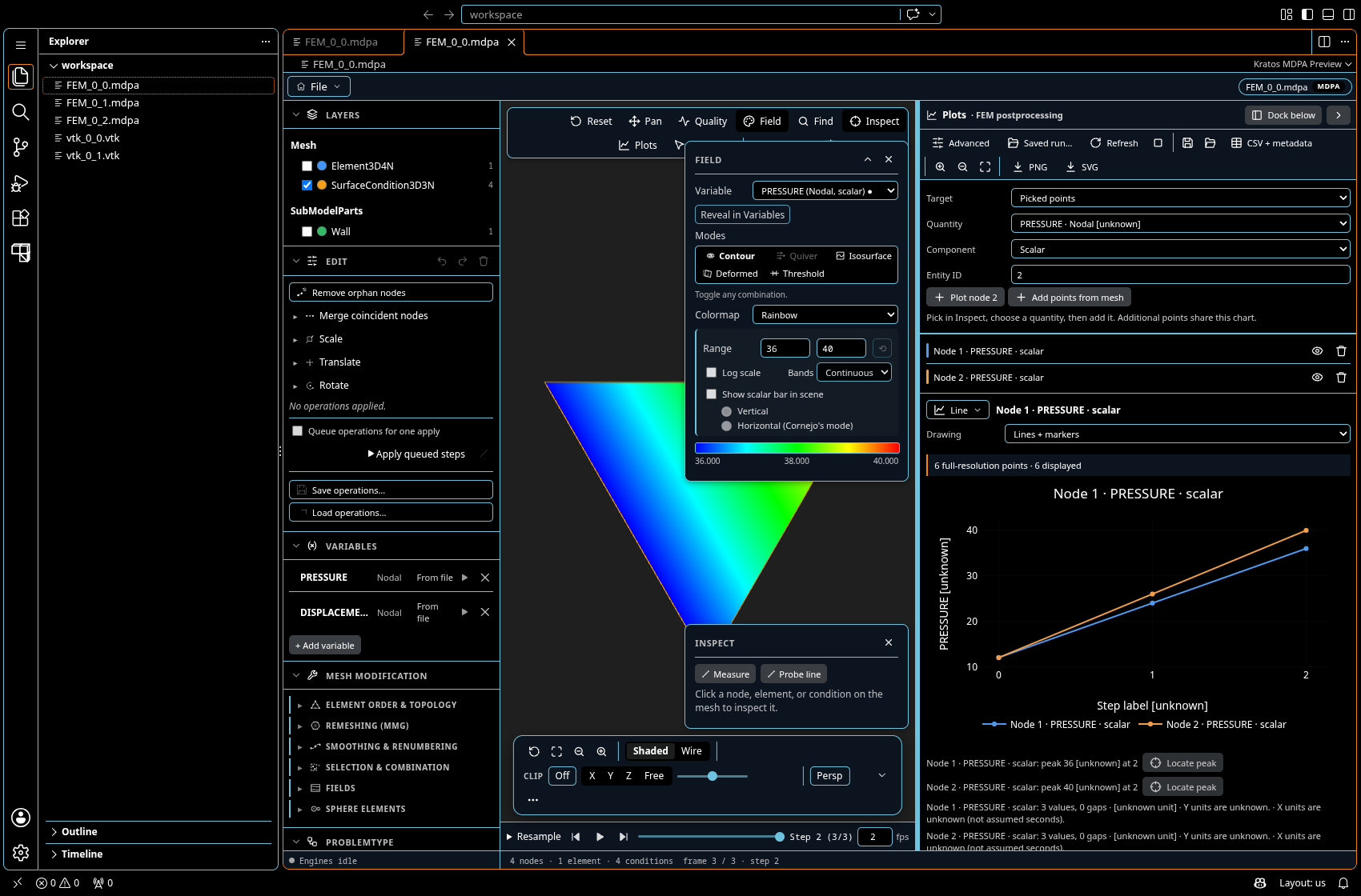
Captured from the packaged extension in code-server, not a mockup. The mesh and chart share one editor: the Quantity dropdown defaults to the displayed field, so tracing the contoured variable needs no reselection. This MDPA fixture supplies neither units nor physical time: axes honestly show unknown units and filename step labels, not Pa or seconds.

Open the workspace

• With a mesh preview open, choose the toolbar's Plots button or Advanced ▸ Plot builder…. Plots opens to the right within that preview, not as another editor tab. Dock below / Dock beside, a pointer/keyboard-resizable separator and Hide / Plots let you adjust or collapse the split without losing curves. Plots and Flowgraph take turns in the auxiliary space; revealing one collapses the other without unloading its work.
• Inspect ▸ Plot over time, and Plot beside a field value, add the entity's history. The Data table, legacy history panel and Probe line panel also offer Plot builder… shortcuts, preselecting their association/history/profile.
• Without a mesh, run Kratos Mesh: Scientific Plot Builder in the Command Palette. Choose Add source, then a CSV/TSV file. The existing empty-mesh preview remains a mesh launcher; it is not required for table plotting.

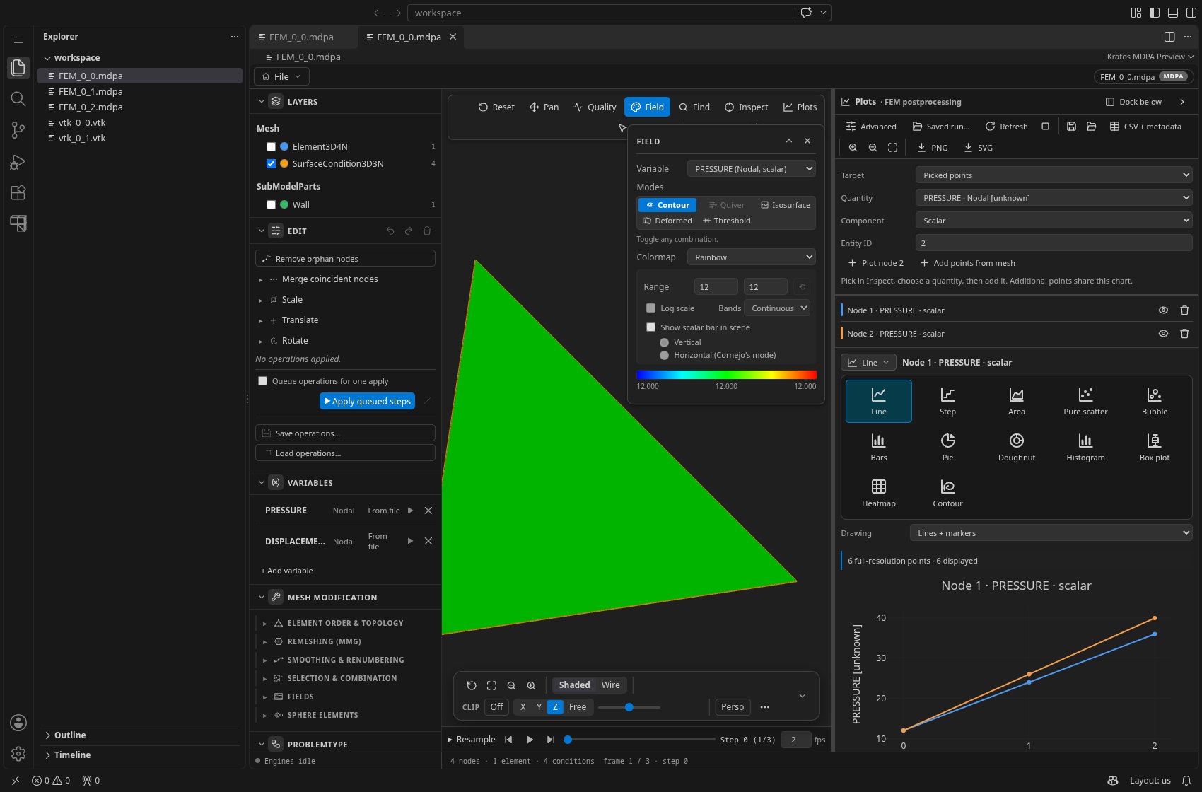
The embedded pane starts with simple Target → Quantity → Component controls; Advanced is hidden until requested and edits the same recipe without clearing its curves. The standalone workspace shows the full configuration column. The Chart type button above the plot opens a labelled visual icon picker in either workspace. Drawing style, bar arrangement/orientation, category statistics and bubble-size mappings are available outside Advanced. Choosing a chart type keeps sources, curves, visibility and profile-following bindings; an incompatible mapping produces a diagnostic, not a silent replacement. Recipe edits update the preview after a short debounce; choosing the next point/region does not rescan existing curves until you add it. Refresh explicitly rereads the source, while Cancel stops the current worker. Icon-only actions have accessible names and hover tooltips.

Point histories and peaks

1. Pick a node/entity with Inspect, then choose Plot beside displacement, pressure or another supplied field. Alternatively enter its Entity ID in Plots. The mesh view stays rendered beside the chart: a displayed field (for example a PRESSURE contour) remains visible while its point history is plotted, so the 3D view and the trace can be read together.
2. Select a scalar, vector component or Magnitude. Choose Plot node… to append it. The Quantity dropdown defaults to the field currently displayed in the focused pane (falling back to displacement, pressure, then the first supplied field), so tracing the contoured variable needs no reselection.
3. For several points, choose Add points from mesh, then click mesh points. Each click appends a history with the selected quantity/component; Done picking or Escape ends this mode. Existing curves stay on the chart, with Hide / Show / Remove controls.

Point and regional requests from the same path scan together, loading each frame once. Missing fields, missing IDs and changed field/time metadata are distinct diagnostics, not zeros. Histories always use disk values, not replayed edits. Locate peak uses the full-resolution maximum even when display samples are reduced, and moves the owning preview to the original frame/entity when ownership is still valid. A point's history peak is not a regional maximum: regional magnitude extrema compute each entity's magnitude before selecting the maximum.

Analyze a SubModelPart

Hover/focus a SubModelPart in Layers and choose Analyze / plot this SubModelPart, or choose Target: SubModelPart / whole mesh and select a Region. The region is highlighted read-only. Choose a supplied field/association, operation and Current frame / Over time, then Add region curve. Current-frame results are bars; histories are lines. The simple workflow refuses to mix those different domains in the same chart rather than silently changing existing curves; remove them before changing scope or use explicit Advanced mappings.

Operation	Meaning and requirements
Minimum / Maximum / Entity mean	Selected component or entity magnitude over unique region members. Mean is unweighted, not an area/volume mean. Extrema retain the responsible entity ID. Whole-mesh reductions are available.
Sum / support reactions	Sum supplied scalar values or vector components. Vector components are summed before any chart magnitude; opposing reactions cancel. Do not use a traction/displacement field as a nodal reaction force.
Boundary mean pressure / Boundary scalar integral	Measure-weighted scalar mean or integral over boundary Conditions. Accepts explicitly selected Nodal or Conditional fields; no implicit Elemental-to-boundary conversion. Scalar integrals need no normal.
Pressure force / Pressure moment	Integrate −(p − pressureOffset) n. Choose Normals: outward / winding and the pressure offset; a moment additionally requires an explicitly entered Moment origin XYZ. Outward normals need exactly one adjacent element; unorientable/internal facets are excluded and disclosed.
Flow / heat flux	Integrate a supplied 2/3-component vector field dotted with the selected normal. This does not infer velocity, density or conductivity from a name or a temperature field.
Measure-weighted total	Sum of a scalar Elemental field times each element's length, area or volume (top dimension of the mesh). Elements with no value or no measure are excluded and reported, never counted as zero.
Reaction moment	Sum (x − origin) × supplied nodal force, with explicit reference coordinates and compatible force dimensions when recorded.

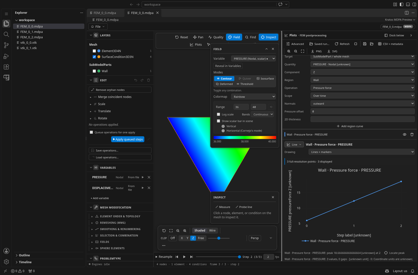
All coordinates are source coordinates, never visually exaggerated deformation. Node-only parts define no integration boundary. By default a boundary operation uses the Conditions of the chosen part. Choosing Boundary: Exterior faces of the region's Elements (Nodal fields only, always outward normals) instead integrates over the faces owned by exactly one Element of the region (or of the whole mesh). A face that is also owned by an Element outside the region is an interface whose side is ambiguous: it is excluded, counted as uncovered measure and reported, never assigned to either side. Two-dimensional line boundaries must lie in the XY plane and are per unit depth unless a positive thickness in the coordinate unit is supplied. Three-dimensional surfaces use area. Unknown coordinate/field units remain unknown; supplied scales such as kPa and mm are preserved as compound labels, not silently converted to N. A recorded SI kinematic-pressure field (m²/s²) needs explicit kg/m³ density for pressure loads.

Triangles use degree-two quadrature for pressure moments; lines use two-point Gauss quadrature. Quads/polygons use a disclosed piecewise-linear triangle fan, and higher-order boundaries use disclosed corner skeletons rather than pretending to perform full isoparametric quadrature. Subtree memberships are deduplicated; separately plotted overlapping regions remain independent. Missing coverage and unavailable regions per frame are diagnosed, not filled with zeros. Units, gaps and a compact coverage summary stay visible below the chart; complete diagnostics remain expandable.

Plot presets

The quick panel's Preset selector builds a complete recipe from a few inputs instead of hand-wiring sources: a field distribution (histogram of a displayed field), a section comparison over time (one curve per SubModelPart), a measure-weighted Elemental total, tensor/vector components by index, tensor invariants (von Mises, principal values, … from a layout you supply), a heat-flux balance through boundary sections, or one table column against another — plus a user-supplied threshold check and from − to section differences on evaluation, and an explicit pressure-density conversion for kinematic-pressure fields. Every preset is a pure recipe builder with no numerics of its own, so a preset curve and its hand-assembled equivalent cannot disagree. See Plot Presets; headlessly the same builders are the plot_preset MCP tool.

Import a table

1. Choose Add source, keep Source type: table, and enter a file path or use Browse….
2. Choose Inspect source to see the first twelve records, row count, stable column IDs and diagnostics.
3. Correct Delimiter and Headers if automatic detection is not appropriate. Comma, tab, semicolon and pipe are supported. Quotes, escaped quotes and multiline cells are recognized.
4. Missing tokens are comma-separated; the defaults are an empty cell, NA, N/A and null. A missing or nonfinite numeric value becomes a gap, never zero. Ragged records are rejected rather than truncated.
5. Numeric columns optionally specifies numeric column IDs such as c0,c1. Invalid cells then become diagnosed gaps. Without an override, a column containing ordinary text is classified as text.
6. Supply units in headers, for example Force [N], or through Units, for example c1=N,c2=mm. Unit text is retained exactly; dimensions are recognized only for the curated names supported by the field-dimensions core. Unknown units are not assumed dimensionless or SI.
7. Choose Add series, then its X/Y columns. Add another series to overlay a second quantity or another file. Column IDs remain distinct even when headers are duplicated.

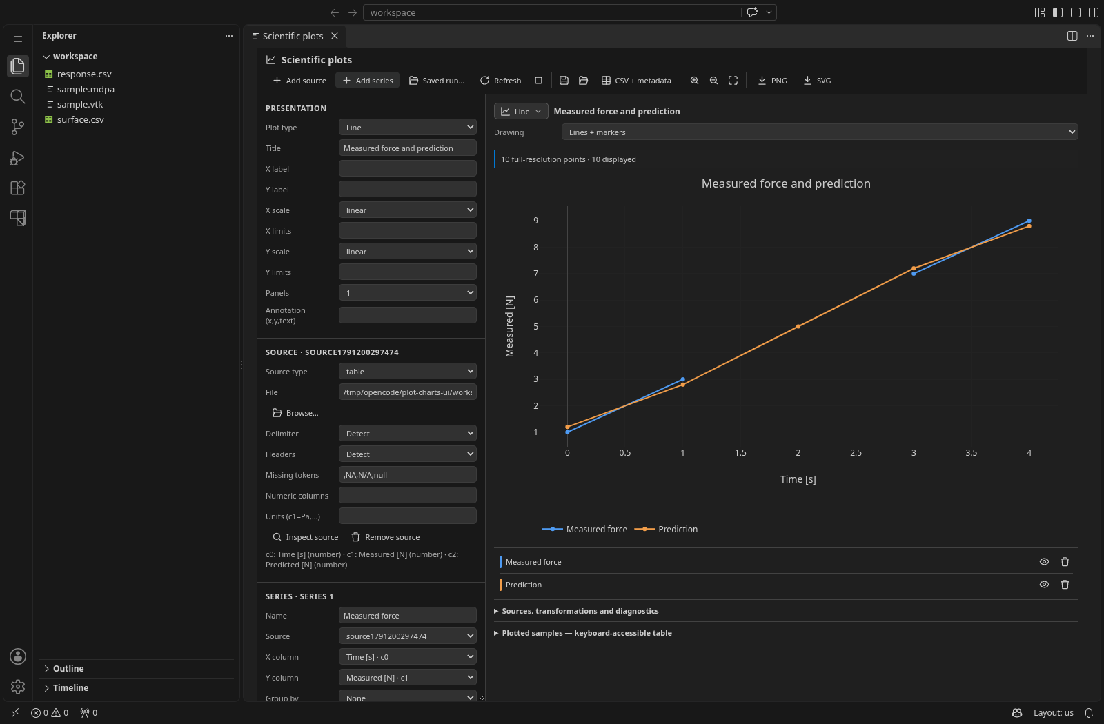
For this standalone screenshot, the table is:

Time [s],Measured [N],Predicted [N]
0,1,1.2
1,3,2.8
2,NA,5
3,7,7.2
4,9,8.8

Simulation sources

Source	Configuration and semantics
mesh	Choose Nodes, Elements, Conditions or Geometries, an optional SubModelPart, selected IDs and an optional frame index. Point and cell ID spaces remain independent. Geometries have no dedicated field association, so overlapping Elemental fields are deliberately excluded. Field mappings are keyed by association, variable and component, not an accidental table position.
history	Choose an association, entity ID and variable. The shared field-series collector discovers steps from the supplied path and reads disk values, without replaying mesh edits. Components appear as separate columns. Filename step labels and frame indices are not physical time; supply one Physical times value per collected frame and a Time unit when known. In-file time values are used only when the source exposes them.
probe	Choose a Nodal field, polyline XYZ points separated by semicolons, sample count and captured Frame index. The shared line-probe extractor returns distance and component columns. Uncovered samples remain gaps; there is no implicit cell averaging. In the owning preview, Follow timeline opts into live frame updates.
region	Choose the field association, variable, region, operation, component and current/history scope; specify normals, offset, thickness, density and moment origin where applicable. The same regional extraction is available through MCP recipes.
inline	A saved snapshot or a table supplied through a recipe/MCP. Its rows and metadata are stored in the recipe itself. It does not claim a live mesh link on reload.

Embedded mesh/probe/current-region requests use the owning provider's actual model, including live edits and resampled frames, unless an explicit disk-run binding is selected. Explicit current-frame sources remain pinned to their captured frame when the timeline moves; Refresh at that frame on the same timeline can capture newer edits. A filename-series disk frame is resolved through that series, not treated as an in-file step. History sources always read disk results. A topology-size change warns that an ID may no longer describe the same physical entity; it is not an automatic remeshing correspondence.

Saved runs and physical-time cursors

Choose Saved run… to discover the existing tracked-run records or choose a saved-run directory. Discovery reads that directory and its immediate child run directories, not an unbounded workspace scan. Select the run and result/rank explicitly. This appends a disk mesh source and opens its configuration; choose its association/columns, or change it to a history/probe/region. Bind saved run… / Rebind saved run… binds an existing source without silently changing another preview.

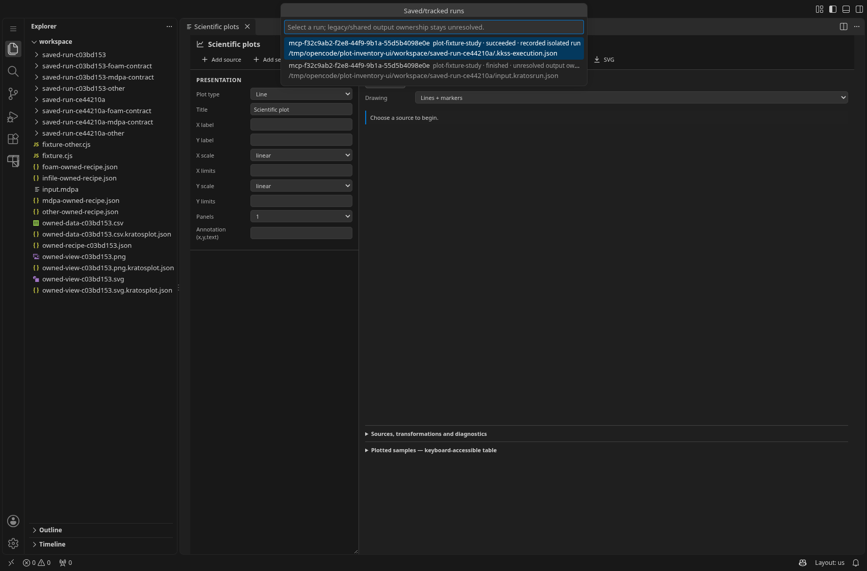
An existing terminal isolated-run .kkss-execution.json receipt must record the owning run, study/request IDs and SHA-256 revisions of the source mesh and results. Binding checks the actual bytes of the selected rank/timeline, filename SubModelPart files and recursive index companions. Collection checks ownership before and after reading; changed/missing sources, companions, source meshes, receipts or timeline entries require explicit rebinding. Terminal receipt revisions are frozen when completion is observed: later status polling cannot adopt rewritten outputs as the old run. A free-form Run label (unverified) does not authorize ownership.

An available latest-run sidecar that names a different run/study/request or a live state also refuses ownership, even if the result bytes are identical. Reloading a recipe preserves its binding, not a promise that its sources are still unchanged.

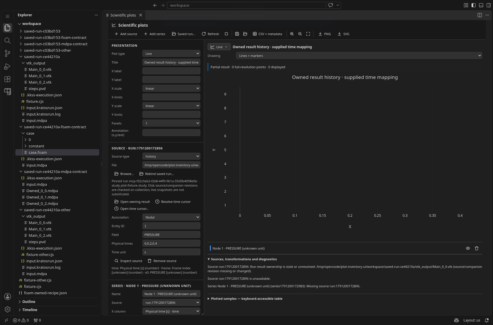
Latest-run sidecars from shared/reused output directories and live/uncertain runs remain unresolved, without adopting matching files. Directory-backed results need more than marker/file hashes: the result artifact must also carry an inventoryRevision frozen by its owner, with each dependency recorded as a result/companion artifact. OpenFOAM covers complete constant/, system/, numeric-time and processorN/ trees, including compressed fields, moving meshes, regions, zones and processor addressing; Elmer covers mesh/binary inputs and partition trees; MFEM rank entrypoints cover the sibling ranks the reader merges. A removed field, added empty region/time directory, changed companion or linked dependency refuses ownership. Inventory coverage does not imply that the reader understands every field or reconstructs every case shape. An old marker-only receipt cannot be upgraded by hashing today's outputs.

Index discovery is bounded to 4 MiB per index, 50,000 files and 20 levels; directory enumeration to 50,000 entries including directories; run records to 8 MiB and discovery to 256 records/64 input paths. These are protective limits, not measured large/remote budgets. Cancellation terminates the verification worker without changing the mesh or run store. The receipt-writer contract describes the shared freezing helper and relocatable closure.

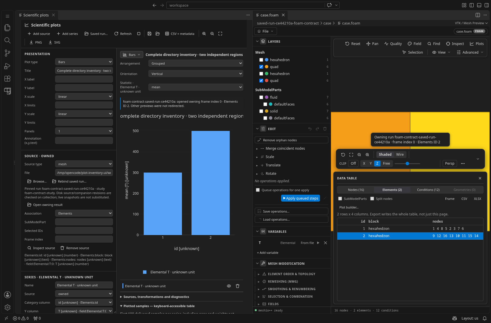
For a bound history/region source, Resolve time cursor matches a supplied time with exact or tolerance-bound nearest matching. Supply Physical times and Time unit for filename series or unknown/different in-file units; times must be strictly increasing, with one value per available frame. Unit conversion is never implicit, and equal-distance nearest matches — including distances equal only within floating-point roundoff — select neither frame. A newer saved-run request, changed source settings or a closed workspace discards a late reply instead of applying it. The notice identifies the owning run and matched frame index; resolution alone does not navigate. Open owning result explicitly opens that run's verified result; Open time cursor… resolves and then opens the exact owning frame.

For a verified sample, a chart click or Show in mesh / Locate peak explicitly opens or reveals the recorded source's MDPA/VTK preview and selects its original-association entity or SubModelPart in the exact recorded frame. Ownership is checked again before and after off-screen frame loading; only then is the model adopted and selection shown. Separate run/source paths use separate previews, never whichever case is active. An edited, resampled, busy, recording or changed preview refuses the handoff, preserving its work. IDs are checked for presence in their original association, not treated as evidence of correspondence between runs or remeshed frames. Unverified run labels and interpolated samples have no owning-run link; bound disk profiles still cannot follow an unverified preview timeline.

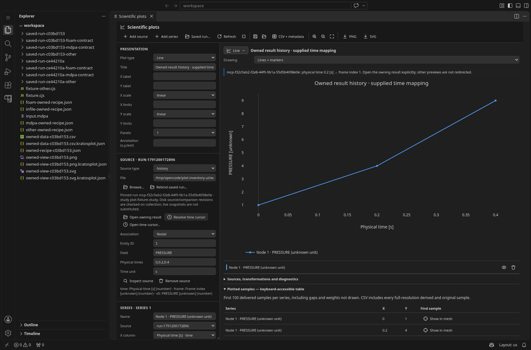
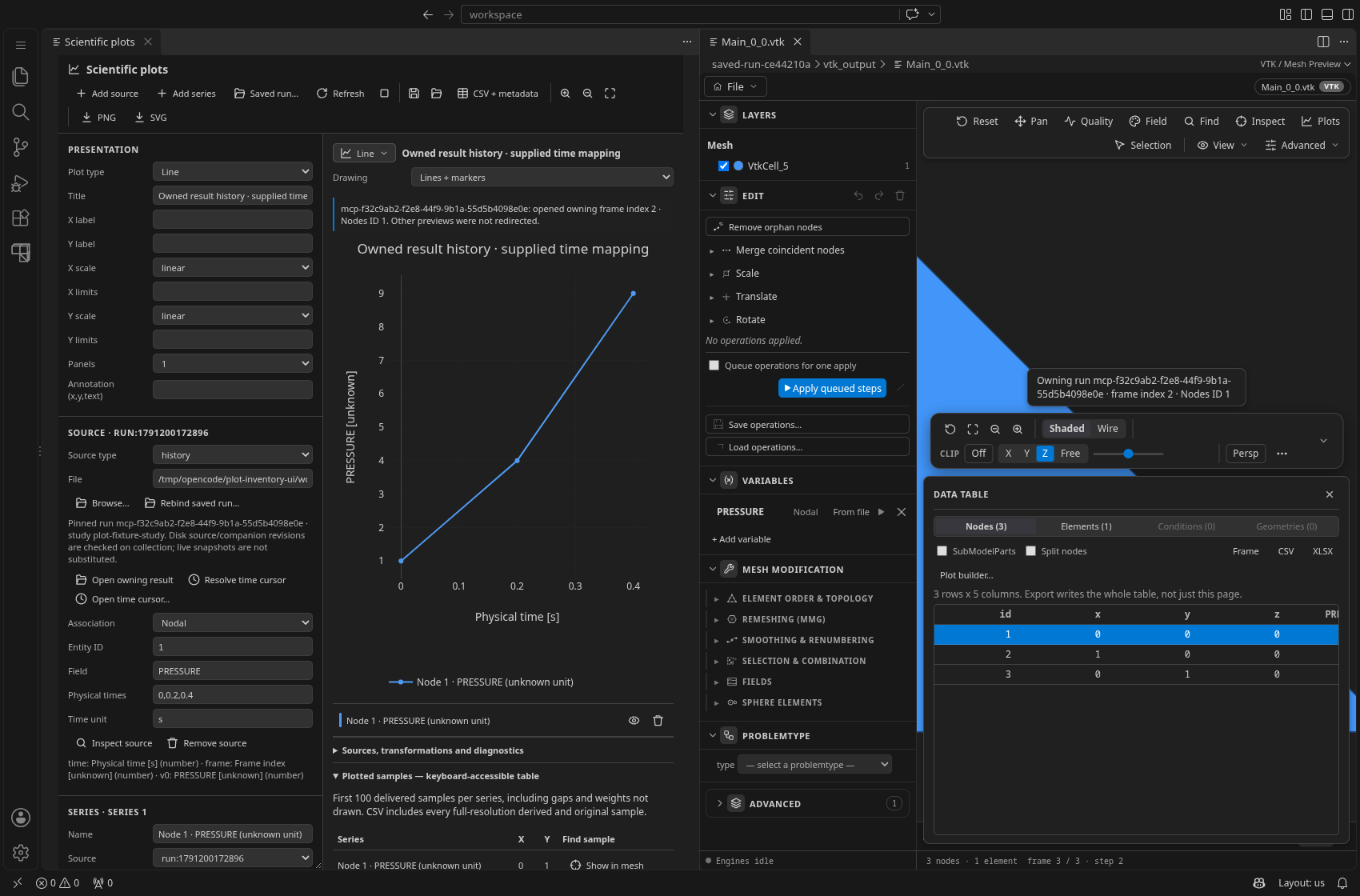
These captures use the installed VSIX and real run-store/provider/dialog flows. The packaged MCP server dispatches Node fixture processes, not Kratos. They write three known result frames and an in-file PVD timeline; the GUI explicitly supplies 0, 0.2, 0.4 seconds. A separate MDPA receipt-contract fixture exercises that provider without claiming solver output. Pressure units remain unknown, and no cross-mesh entity correspondence is claimed.

Follow a spatial profile

Open Probe line ▸ Plot builder…, or configure a probe in Advanced. Profiles start fixed. Their curve row shows the captured frame; choose Follow timeline to resample the same spatial coordinates as this preview steps or plays. Fix frame retains the current profile for comparison with another following curve. This does not infer material-point motion or sample the viewport's exaggerated deformation.

Only followed probes change during frame updates. Unchanged sources use bounded session-only extraction snapshots, so scrubbing does not rescan disk histories or change a fixed curve's values. Numerical transformations and comparisons are reevaluated against those retained samples. Refresh explicitly rereads sources; this snapshot retention is not a file-change-aware cache. If a fixed extraction was evicted or cancelled, following stops with an actionable Refresh diagnostic instead of secretly rereading it.

Changing the timeline, rank or resampling configuration pauses following and keeps fixed snapshots. Resume following explicitly binds the profile to the new timeline, including its provider-owned resampled model. Cancel also pauses following until resumed. A frame change during collection is coalesced to the latest frame after the current collection completes; late results cannot replace a newer request. Saving a live profile embeds the captured table, not an auto-following link to whichever mesh happens to be open after reload. Headless/MCP probe recipes always sample their explicit timeStep; followTimeline is UI intent, not an instruction to discover an active preview.

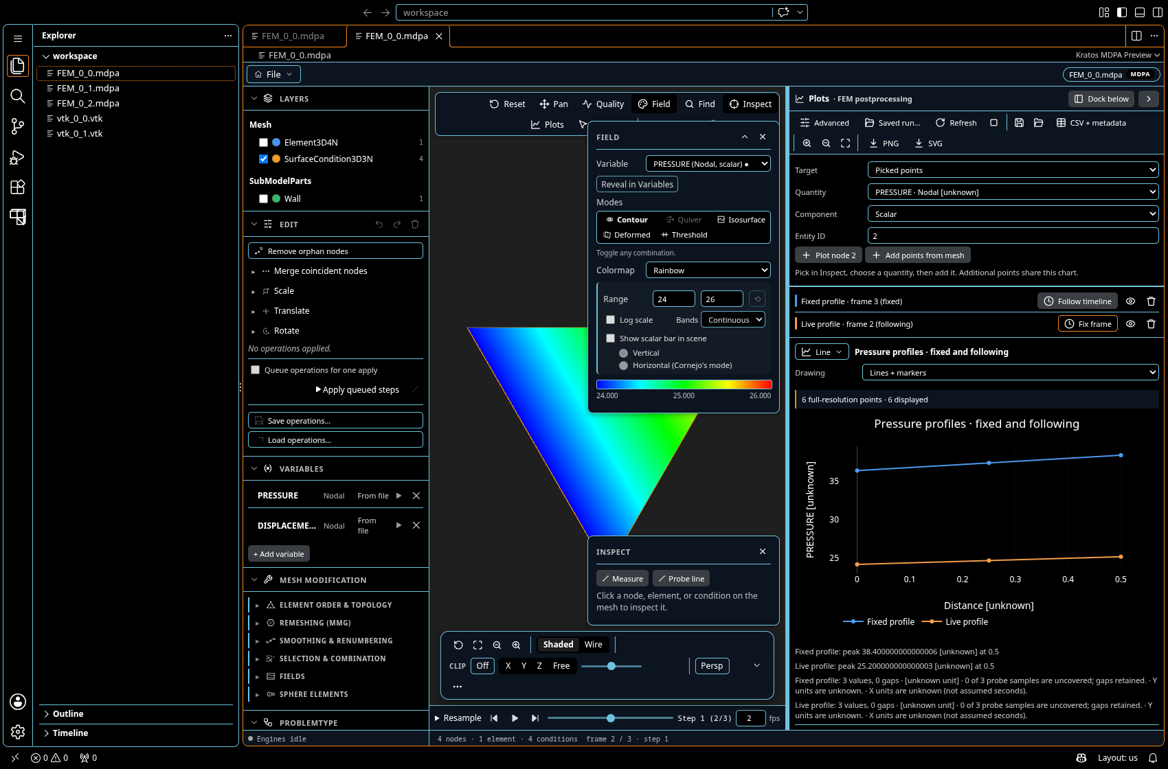
The fixed curve retains frame 3 while the live curve samples frame 2, shown by the owning mesh. This fixture supplies no coordinate or pressure units. Frame numbers are not seconds, and interpolated spatial samples do not claim invented entity links.

Families and analysis

The visual picker exposes thirteen families, including Polar (X column is the angle in the unit you choose explicitly, Y column the radius). “Graphs” here means ordinary data charts, not a node-and-edge network editor. X and Y can represent any appropriate relationship, including force–displacement. A series can be split by a grouping column; multiple sources/series support histories or file comparisons.

View	Controls and meaning
Line	Drawing: Lines only / Lines + markers. Existing recipes retain line+markers by default. Missing values break lines.
Step	Horizontal then vertical: hold each value to the next X sample. This is a display convention, not inferred temporal interpolation.
Area	Fill each covered interval to zero. Missing intervals use separate fill polygons; this is neither a computed integral nor an uncertainty band.
Pure scatter	Markers only, without connecting lines.
Bubble	Markers whose area is proportional to a supplied numeric Size column. No size is inferred from Y.
Bars	Choose mean/sum/min/max/count, grouped or signed stacked, vertical or horizontal. Stacking adds compatible values but does not prove disjoint regions.
Pie / Doughnut	Per-category shares, with an explicitly selected statistic, nonnegative weights and a finite positive total. Each curve is a separate circular chart.
Histogram / Box plot	Host-computed equal-width bins or quartiles/Tukey whiskers; a distribution is not supplied uncertainty.
Heatmap / Contour	XYZ samples with explicit regular/nearest gridding and masked uncovered regions.

Pie and doughnut shares

Select Pie or Doughnut, map Category column (the series' X mapping) and numeric Y column in Advanced, then choose Statistic · curve name above the chart. There is deliberately no automatic pie statistic: repeated category rows might represent contributions to sum, finite observations to count, or values to average. Mean/min/max are also available but describe shares of those chosen statistics, not conserved physical totals. Count counts finite selected Y values, including signed input values; other statistics refuse negative contributors rather than taking absolute values. Supplied conversions and row filters remain explicit and are recorded before aggregation.

Missing categories/values are reported, all-missing categories remain gaps, and zero weights have no slice. Missing categories are excluded from the denominator, so the shares describe covered weights only, not complete coverage of an unknown physical whole. Zero-total/overflowing weights are refused. Category values, their total and dimensionless share fractions are host-computed and available through MCP/CSV; original selected rows remain available separately. Aggregation does not invent entity correspondence or uncertainty propagation. Category charts are capped at 1,000 categories without silent truncation; circular shares are never display-sampled.

Multiple curves appear as separate pies/doughnuts, with common supplied units required within a panel. Overlapping SubModelParts are not automatically an exclusive partition, and no regional membership is inferred from a label. Circular charts have no Cartesian axes; log scales are refused, and retained XY limits/annotations are diagnosed as not drawn.

Slice labels display the host-computed shares, and matching category labels keep matching colors across circles. Category legends are keys, not hide/re-normalize controls: use an explicit row filter to change the denominator, or the curve-row visibility button to hide a whole circular chart.

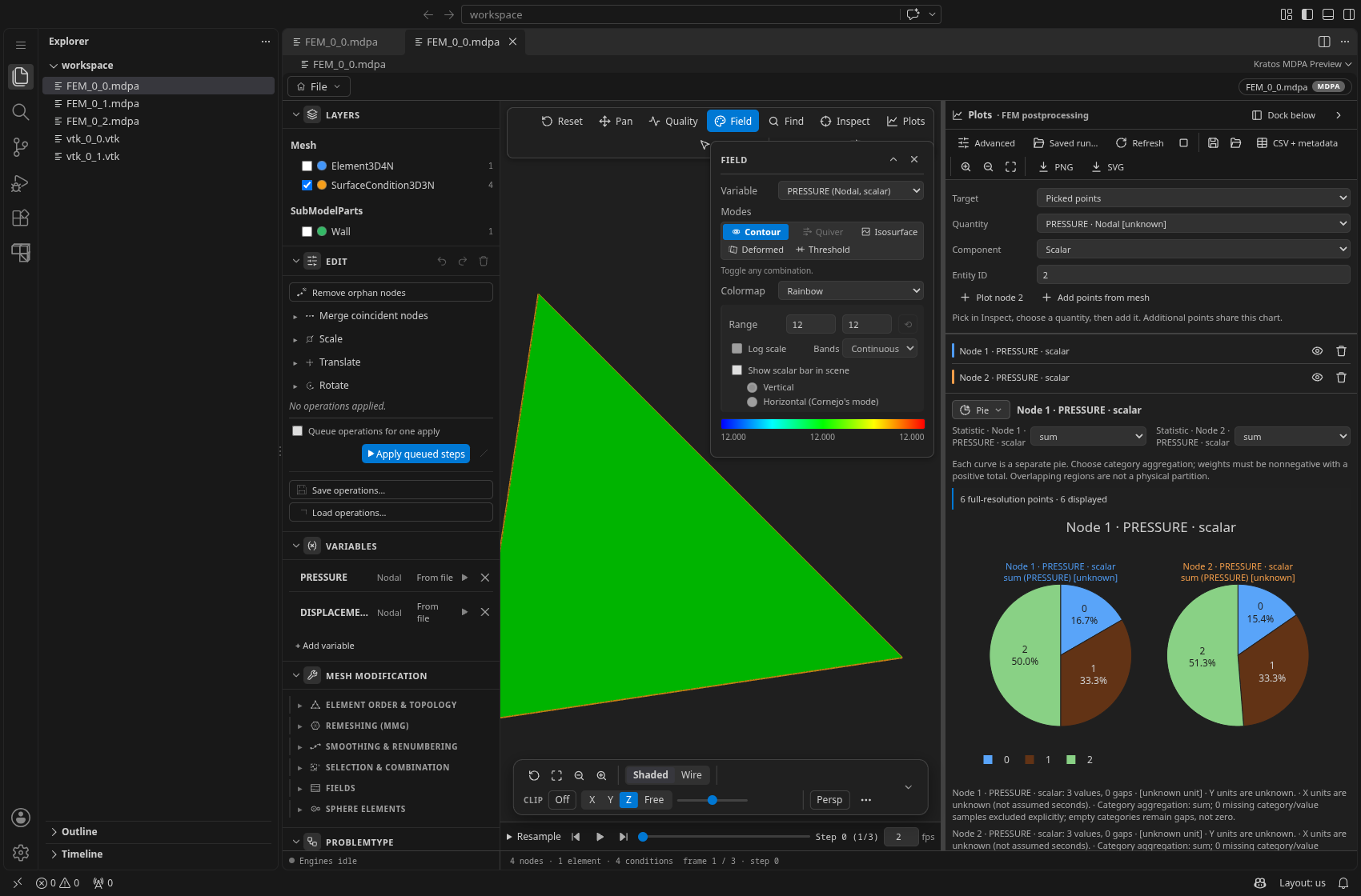
This packaged MDPA fixture supplies unknown units and filename step labels. These circles show shares of explicitly summed sample weights within each history; they are not time integrals, verified forces or fractions of a disjoint mesh region.

Bubble sizes

Select Bubble, then explicitly choose Size · curve name. The size column must be numeric; its supplied unit stays visible in hover/export metadata. Negative, missing and zero sizes are not drawn, while the original signed/missing samples remain in numeric exports. Maximum diameter px in Advanced sets the visual scale (4–100 px, default 36); the full-resolution maximum controls that scale even when points are display-sampled. Size values do not undergo the series' Y transforms, and alignment does not invent interpolated size weights.

• Magnitude columns lists explicit numeric component IDs in the same units. Individual components use the normal Y picker.
• Filter accepts column,min,max. Recipes/MCP additionally support an exact text-value filter. Removed rows are outside the selected analysis; missing rows inside the selection remain gaps.
• Histograms have explicitly configurable equal-width Bins. Grouped bars select mean, sum, minimum, maximum or count. Box plots use linearly interpolated quartiles and whiskers at samples within 1.5 IQR; a distribution is not an uncertainty estimate.
• Add analysis builds an ordered list. Smoothing uses a centered, odd-sized moving window, clipped at segment ends. Regression reports slope, intercept and R². Derivatives use neighboring secants with one-sided endpoints; integration uses cumulative trapezoids, restarting after each gap. Calculus requires strictly increasing numeric X within each covered segment; sorting and duplicate removal are never hidden operations.
• Normalize divides by an explicitly supplied value in the input Y unit. Convert multiplies by an explicit positive factor and supplies a target unit; changing physical dimensions is refused. Equal dimensions alone do not make Pa and kPa numerically interchangeable. Compound derivative/integral labels preserve source scale, such as (kPa)/(ms), rather than silently relabelling values as SI.
• Errors accepts column,meaning, for example c3,instrument standard uncertainty. The error column must use the same supplied Y unit. Negative/missing errors are not drawn. Smoothing, fitting and calculus do not invent uncertainty propagation; raw supplied errors remain available in the original samples.

Sources, transformations and diagnostics shows parameters, counts, missing values, means, population standard deviations and regression coefficients. Statistics and numeric exports use the full dataset, not display samples.

Heatmaps and contours

Choose numeric X, Y and Z columns and an explicit Grid method. regular maps coordinate pairs to a rectangular array and masks missing cells; duplicates are rejected. nearest requires grid dimensions and a positive coverage radius. It masks cells outside the samples' convex hull or farther than that radius from a supplied sample. It is not a triangulated finite-element interpolation or a guarantee that an arbitrary geometric hole is detected. Duplicate coordinates must be resolved in the input; very expensive grids are refused with a budget diagnostic. No scattered sample set is silently interpreted as a regular surface.

Reference comparison

Choose a Reference series, Match method and Tolerance. Exact matching keeps only shared X values. Nearest and linear matching are tolerance-bound, do not extrapolate and do not linearly interpolate across a recorded gap. The reference must resolve to one ungrouped series. Alignment uses snapshots of the reference before alignment, so list order does not change the results. Step labels and frame indices are refused as a physical-time alignment axis. Unit/type mismatches require explicit correction or a separate panel, including a known unit mixed with an unknown one.

Interpolated points do not acquire invented entity/frame identities. An original entity/history sample can be selected through the chart or Show in mesh in the accessible sample table when it belongs to the owning preview. Links are refused for another file, reloaded inline snapshots, an explicitly supplied run ID or a changed timeline. Retained fixed snapshots cannot navigate a replacement timeline, even if its frame indices and entity IDs match. Disk histories cannot navigate a resampled timeline. Automatic cross-run navigation is not yet delivered.

Presentation, keyboard and themes

Set a title, axis labels and limits, linear/log scales, series colors, marker shapes, visibility and 1/2/4 panels. Add an annotation as x,y,text. Nonpositive values on log axes are diagnosed, retained in CSV and drawn as gaps. Categorical X does not support a log axis.

Use pointer drag/hover and the chart toolbar for exploration, or the keyboard-focusable Zoom in, Zoom out and Reset axes icon buttons. Open Chart type, use arrows/Home/End to move between labelled chart buttons, Enter/Space to choose, and Escape to close and restore trigger focus. Standard controls support Tab and Shift+Tab with visible focus. The expandable Plotted samples table gives keyboard-accessible values and entity-selection buttons for the first 100 displayed samples per series. CSV contains all values. This is an accessible alternative to the chart, not a claim that every Plotly gesture is keyboard-accessible. Pie/doughnut views have no axes to zoom; resize the pane to enlarge them.

Save recipes and export

Save recipe writes version-1 JSON with sources, mappings, ordered transformations, comparison parameters and presentation. Disk and run-receipt paths are relative to the recipe's directory. Pinned disk-run bindings survive recipe reload and are verified again; they are not replaced by the current live mesh. Live mesh/probe/current-region snapshots are embedded as inline tables so reloading does not substitute unedited disk values. Load recipe validates the version before replacing the current configuration. Missing files/fields identify the source and affected series in diagnostics; other available series can still produce a labelled partial result.

• CSV + metadata writes all derived and original selected samples, including units, source ID/row, entity association/ID, SubModelPart, frame, supplied time and run ID where available. Bubble size/size_unit and circular share columns are appended without changing the existing column order. Grid exports also include every derived grid cell, including masked cells. <output>.kratosplot.json records the recipe, source revisions, statistics, transformations, size scale/category total and diagnostics.
• PNG / SVG export the currently displayed chart, including its visible series and zoom, with a provenance companion. The graphic may use disclosed display sampling; CSV does not. The image manifest records the displayed view separately from the numerical recipe.
• Exports cannot overwrite a source file, or a bound run's receipt, input mesh or recorded artifacts/companions (including symlink aliases). Plotting, styling and saving a recipe do not dirty mesh geometry.

Execution limits and current boundaries

Collection runs in a host worker. Histories periodically publish partial datasets, with statistics over the samples published so far. Cancellation hard-terminates that worker, including a synchronous parser call, and retains its last published partial dataset. If nothing has been published, it returns an explicitly partial empty result rather than presenting unfinished calculations as complete. Source/recipe changes invalidate the old result immediately; late replies do not replace a newer chart or authorize an old export.

Tables are bounded to 1,000,000 rows, 256 columns and a 128 MiB file budget; histories to 5,000 frames; nearest grids to 256×256 cells and an operation budget. The workspace caches parsed table extraction under a conservative 64 MiB budget, checking source bytes and import settings on every refresh. A separate conservative 64 MiB session-retention budget holds fixed extractions for frame-following updates; explicit collection, source inspection or cancellation invalidates that retention. These are cache estimates, not a total host-memory budget. The opt-in kratos.plots.persistentCache setting (also plot_dataset's cacheDir and KRATOS_PLOT_CACHE_DIR for MCP) additionally keeps a bounded on-disk cache of mesh, probe, regional and history extractions across restarts — reused only while the source, its companion files and its timeline have exactly the content they were built from; live snapshots and fixed profile-following snapshots are never cached on disk. File changes are picked up on refresh, not by an automatic plot watcher.

Long line/step/area/scatter/bubble displays use ordered bucket sampling with first/last samples and Y extrema; bubbles additionally retain bucket size maxima. A bucket containing a gap is masked conservatively rather than bridging it. Statistics and CSV are computed first at full resolution. Pie/doughnut category weights are never sampled, so displayed shares cannot change through sampling. Boxes use host-computed quartiles; heatmaps/contours retain their bounded grids. The status line and diagnostics disclose sampling.

Delivered: section comparison, volume total, table-column relationship, section differences, the threshold check, tensor-component, tensor-invariant (supplied layout) and heat-flux presets, explicit pressure-density conversion, exterior-boundary extraction (boundary: "exterior"), and the opt-in persistent companion-aware extraction cache. The installed-VSIX acceptance matrix grew on 2026-10-21: ownership resolution (plot_run_resolve: verified, unverified, unresolved), changed and missing PVD→PVTU→VTU companions, Plot distribution, Show on mesh, the volumeTotal and sectionComparison presets, the whole-mesh exterior-boundary integral, the persistent-cache hit, and a million-row table cancelled, superseded in flight and disposed mid-collection all run against the packaged extension. Still open for roadmap acceptance: explicit resolution of legacy/shared-output ownership, broader geometry conventions, million-row/Remote-SSH memory and latency budgets (no real desktop VS Code, Remote-SSH or KKSS session was available for those measurements, so they are unverified rather than accepted), and the remainder of the packaged recipe/export/timeline regression matrix. The library decision and verification record distinguishes measured behavior from these remaining claims; this increment does not close roadmap item 19.

MCP parity

plot_table_read inspects a CSV/TSV path with the same import options and revision metadata. plot_preset builds a named recipe — field distribution, section comparison, measure-weighted total, tensor components, tensor invariants, heat-flux balance or table relationship — and optionally evaluates it with a threshold check and section differences; see Plot Presets. plot_dataset evaluates a version-1 recipe, including region sources, using the same worker/extractors/numerical core and optionally writes the full CSV plus provenance companion. JSON replies default to 100 rows/points and are bounded to 10,000 per series; totalPoints and fullCount disclose truncation. Inline source rows are not echoed a second time: those replies provide recipeMetadata and inlineDataInRequest: true, rather than a misleading executable recipe with truncated rows. Keep the original request recipe, or use the complete export manifest, for reproduction. MCP cancellation/progress is passed to the worker. mesh_capabilities.plotting publishes supported sources, regional operations, families, transformations and budgets. Styling and interactive layouts do not add numerical operations.

plot_runs discovers the same existing records; plot_run_resolve (read-only ownership resolution: verified, unverified snapshot or unresolved) and plot_run_bind returns the verified run object for a mesh/history/probe/region source. plot_time_cursor takes that binding, result path, time/unit, optional supplied times, exact/nearest rule and tolerance. It returns the owning run and matched frame, or matched:false with an unmatched/ambiguous diagnostic, without manipulating any preview. Receipt/source changes fail verification rather than resolving through the active case.