Mesh Editing & History

The preview is not read-only: the Edit and Mesh Modification sidebar sections apply in-place operations to the loaded mesh, all recorded into an undoable, replayable operation history. The edited mesh is what File ▸ Save / Export writes to disk.

Linear → Quadratic

Convert Linear → Quadratic (Mesh Modification) inserts mid-edge nodes to raise every linear cell to its quadratic ("serendipity") counterpart:

Linear	Quadratic
Triangle2D3	Triangle2D6
Quadrilateral2D4	Quadrilateral2D8
Tetrahedra3D4	Tetrahedra3D10
Hexahedra3D8	Hexahedra3D20
Prism3D6 (wedge)	Prism3D15
Pyramid3D5	Pyramid3D13
Line2	Line3

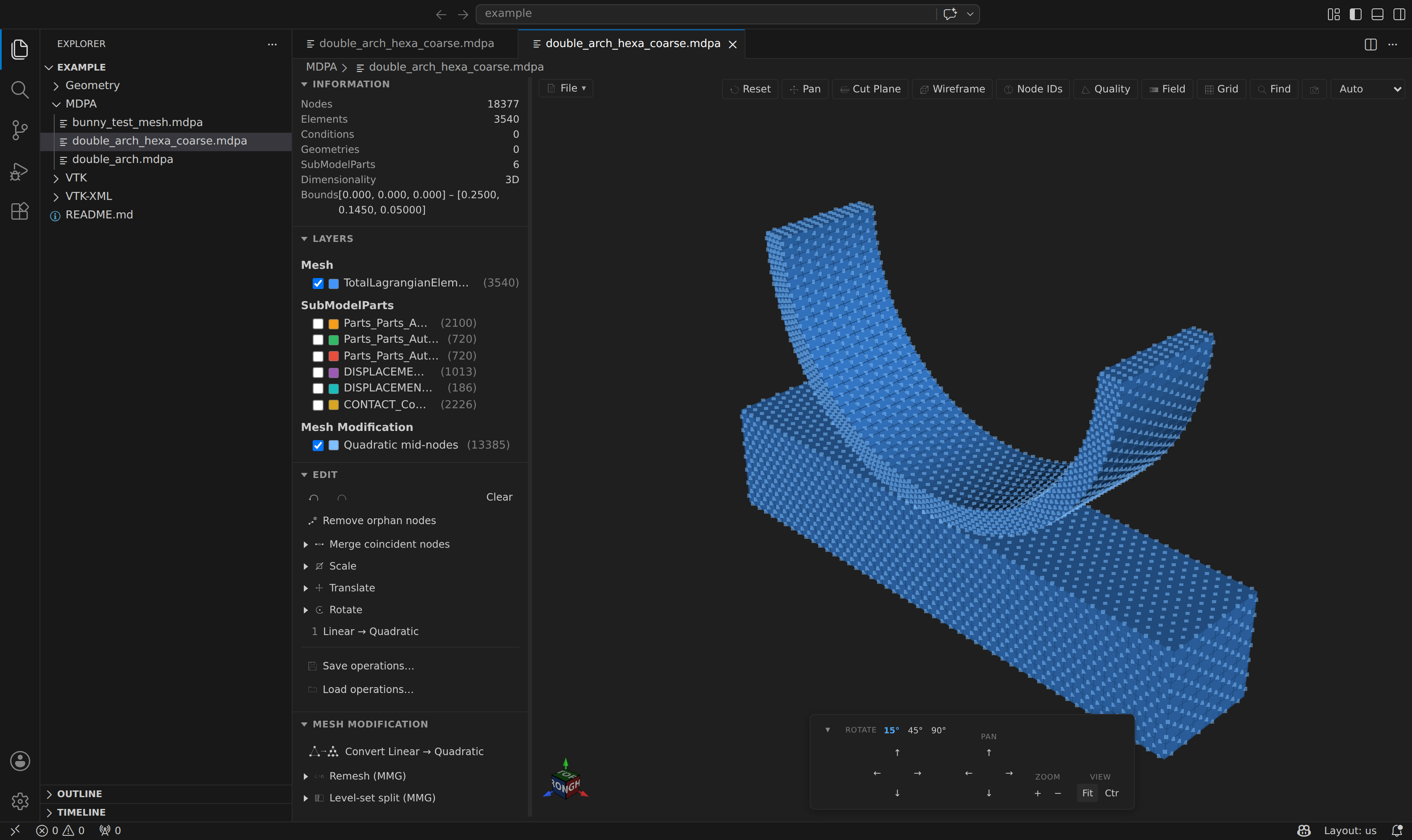
Adjacent cells that share an edge get a single welded mid-edge node, nodal fields are interpolated at the new nodes, and SubModelParts are extended with the mid nodes of their fully-enclosed edges. Cells that are already quadratic or have no quadratic counterpart are left untouched. The new mid nodes are drawn as a semitransparent Quadratic mid-nodes overlay (a toggleable outline row), so you can see exactly what was added.

For MMG-based remeshing and level-set splitting, see MMG Remesh & Level-set.

Additional mesh operations

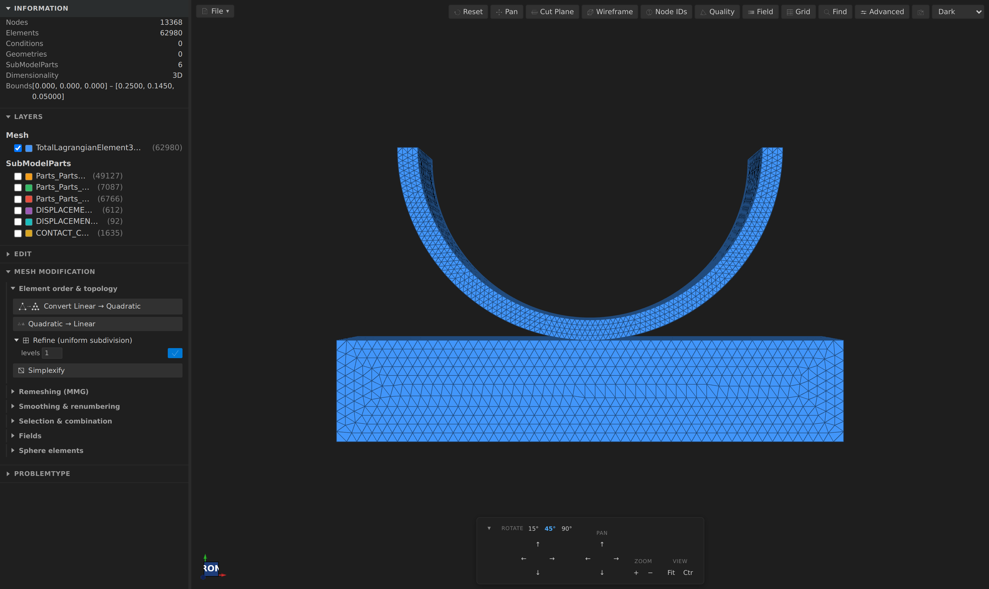
The Mesh Modification section also surfaces the extension's bundled meshio++ as an oracle — it computes something (moved coordinates, a node permutation, a per-cell label) that gets applied onto your own mesh, so SubModelParts, ids and material assignments are never lost the way a raw meshio++ round-trip would lose them — plus several operations implemented natively. These, together with Convert Linear → Quadratic, Remesh (MMG), Level-set split (MMG) and Set element radius, are grouped into six collapsible subcategories — Element order & topology, Remeshing (MMG), Smoothing & renumbering, Selection & combination, Fields, and Sphere elements — so the section reads as a short list of categories rather than a long flat list of forms:

Smooth, Reorder, Partition and Merge mesh run asynchronously — the same inline progress bar and play/stop cancel button as the MMG operations. The rest apply instantly. Every one of these joins the same undoable operation history and JSON recipe as the operations above, and is reachable from the mesh_transform tool on the MCP server, same as every other mesh operation, for scripting.

Reading the screenshots below

Where an operation changes geometry or topology, the shot places the mesh before it (blue, left) next to the result (orange, right) in one view, with the operation's own form open in the sidebar showing the exact parameters that produced it. Where it instead produces a field, the shot colours the result by that new variable through the Field panel.

Element order & topology

Refine

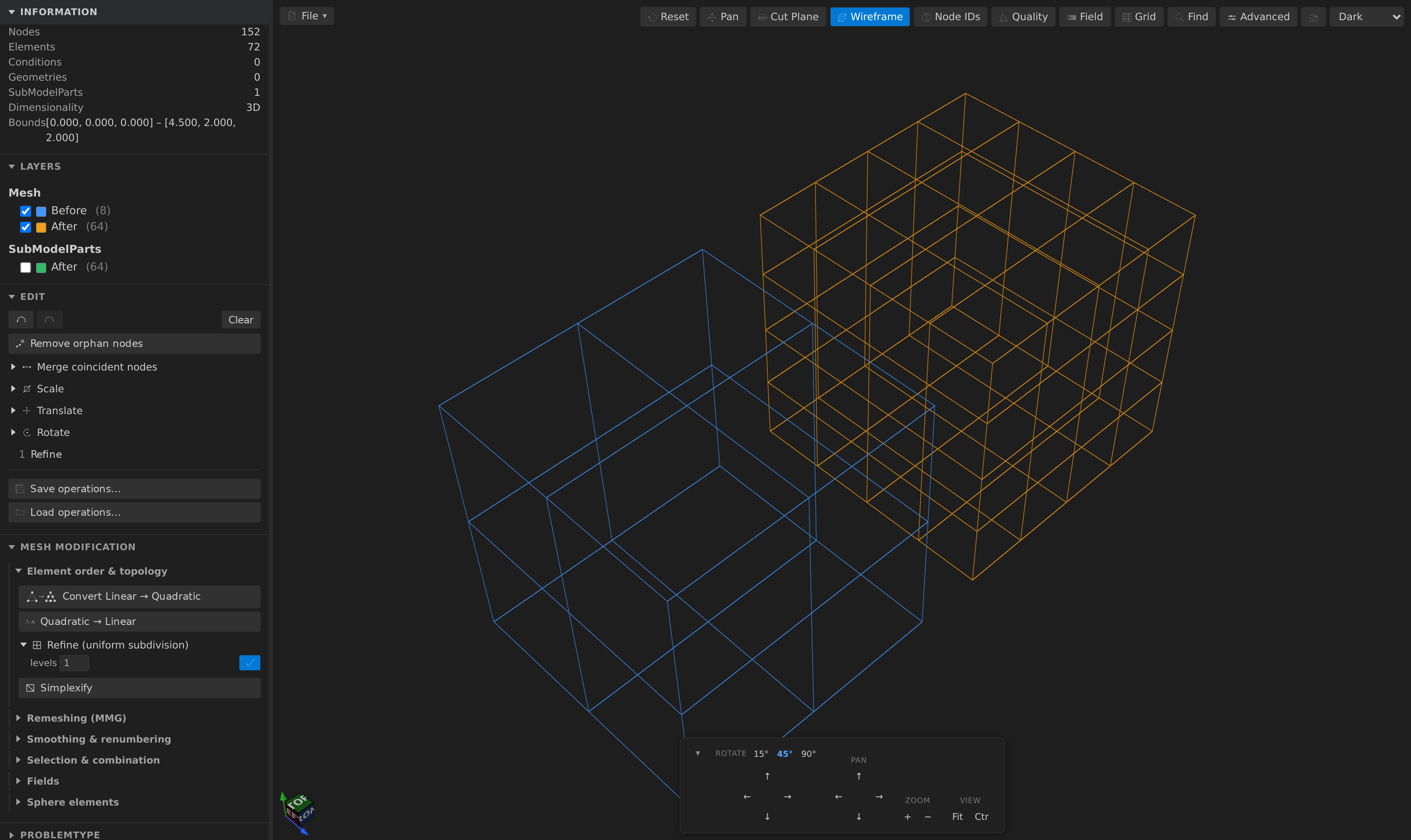
Uniform subdivision: triangles/quadrilaterals/tetrahedra/hexahedra/wedges split into 4 or 8 children, lines into 2, up to 4 levels. Shared edges and faces are deduplicated to a single new node — so there are no hanging nodes — nodal fields interpolate exactly at the new nodes, and elemental/conditional fields and SubModelPart membership extend to the children. The 8 elements above become 64; a second level would make it 512, which is why the level count is capped.

Where chooses what gets refined:

• whole mesh — the uniform behaviour above, unchanged.
• marked by a field — only the cells whose per-cell field passes a comparison. It defaults to ERROR_MARKED > 0.5, which is exactly what Error estimate writes, so estimate the error, then refine where it is needs no extra step. Any per-cell field works: `ERROR_INDICATOR

  0.01` is just as valid, and needs no marking policy at all.

• a SubModelPart — that part and its whole subtree. "Refine the boundary layer" without touching the rest.

Refining only part of a mesh normally leaves hanging nodes — a node sitting in the middle of a neighbouring element's edge, which most solvers refuse. They are resolved for you: a neighbour that inherits a refined edge is given the smallest partial split that keeps the mesh conforming, and that split spreads until nothing is left dangling. The operation reports how far it had to spread.

Selective refinement is simplex-only

Triangles and tetrahedra. Boundary lines and triangles follow the volume they bound automatically, but a mesh of quadrilaterals, hexahedra or wedges is refused by name — there is no partial split of a hexahedron that stays a hexahedron. Run Simplexify first, or refine the whole mesh.

Cells that took a partial split are transitional, and repeatedly splitting one partially is what degrades element quality. They are flagged, and a later refine splits them fully instead — so an estimate → refine → estimate → refine loop stays well-shaped without you tracking anything.

Quadratic → Linear

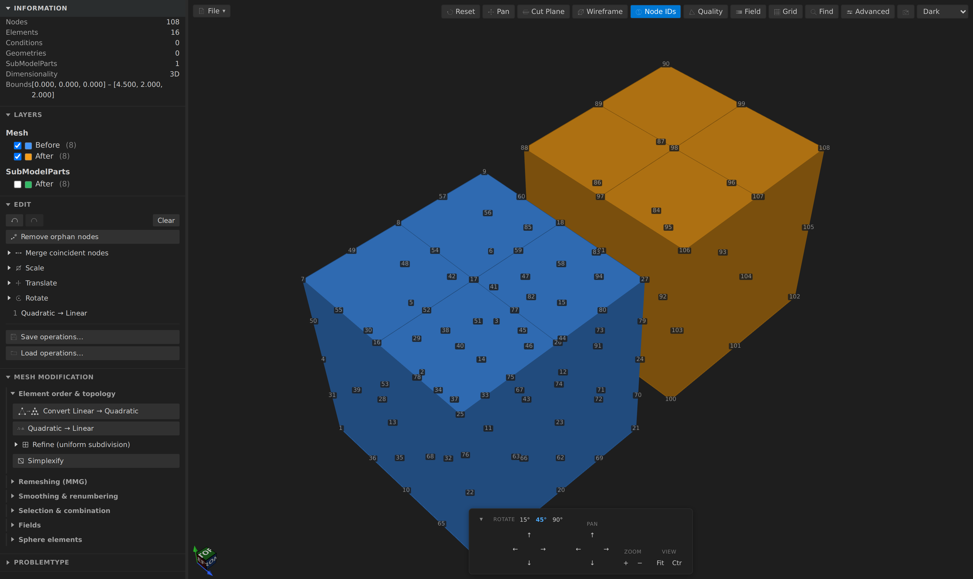
The inverse of Convert Linear → Quadratic: drops the mid-side nodes and restores the underlying linear cell type (Tetrahedra3D10 → Tetrahedra3D4, Hexahedra3D20 → Hexahedra3D8, …), then removes whatever is left unreferenced. With Node IDs turned on the difference is literal — the same 8 cells, 81 nodes before and 27 after.

Simplexify

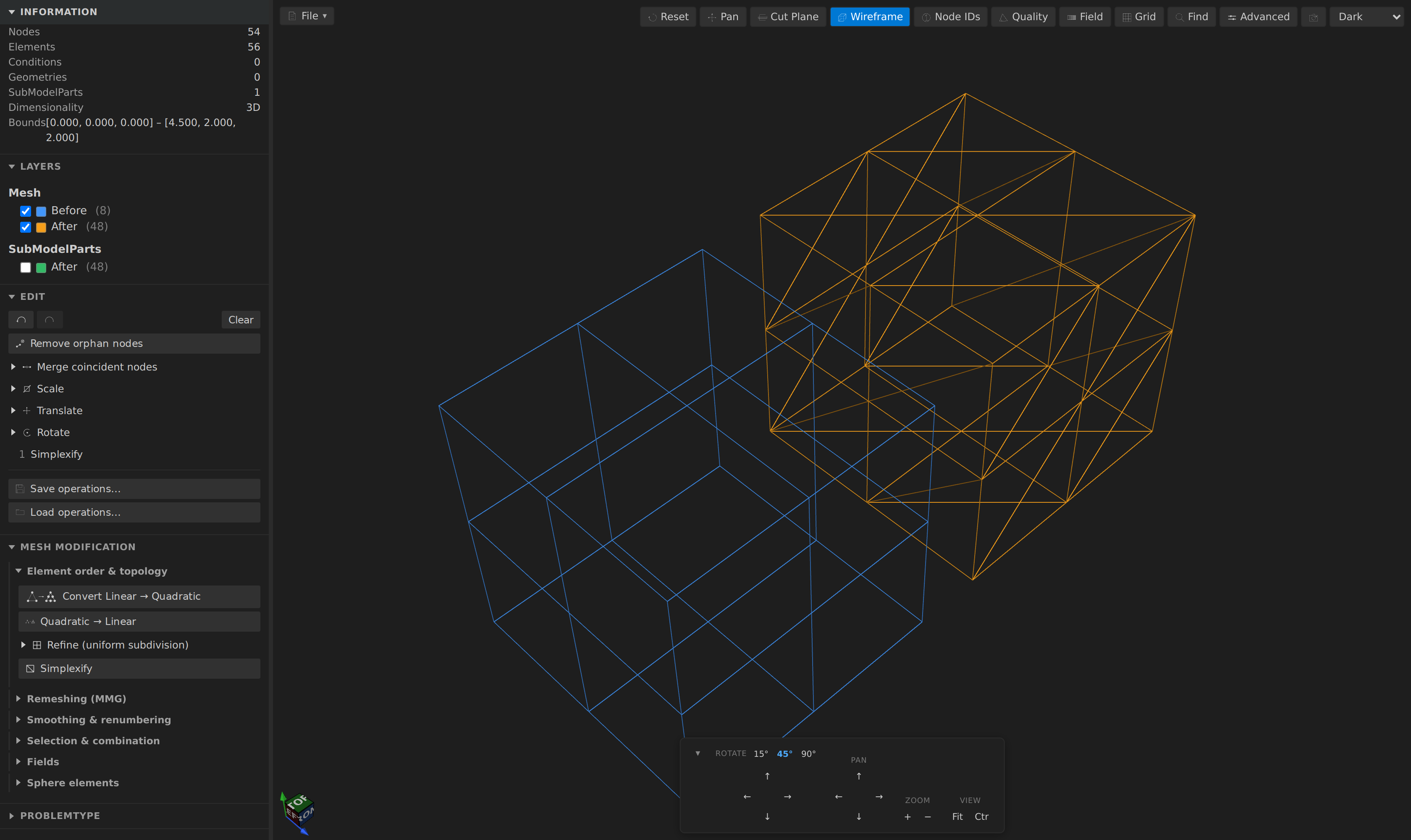
Converts non-simplex cells to simplices: hexahedra → 6 tetrahedra, wedges → 3, pyramids → 2, quadrilaterals → 2 triangles. The first child keeps the parent's id and its siblings get fresh ones, with elemental/conditional fields and SubModelPart membership replicated to each. A mesh that is already all-simplex is a no-op.

Repair surface

Repairs a surface mesh (triangles and quadrilaterals) in place, through meshio++'s repair, as one undoable step. Each fix has its own switch:

• fix winding makes neighbouring faces agree, so no face is wound against the one beside it;
• orient outward points each closed component's normals out of it (it does not infer nested cavities — an inner shell is oriented like any other);
• fill holes triangulates every bounded hole with at most max hole edges rim edges and leaves larger ones open, reporting how many;
• split non-manifold vertices separates two fans of faces that touch at a single point, so each fan owns its own node (non-manifold edges, where three or more faces meet, are counted but never split);
• weld merges points closer than the tolerance first (0 leaves the points alone).

Entities the repair does not touch keep their ids, kinds, property ids, SubModelParts and field values. The faces it creates have an explicit policy rather than an accident: they join the source block of the same cell type — so the block keeps a real Kratos type name — are listed in a new Repair_Fill SubModelPart (suffixed _2… if that name is taken), take that block's most common property id, and carry no elemental or conditional field values (a gap, never 0); nodal fields reach the new hole-centre point as the mean of the hole's rim. The result message reports the boundary / non-manifold / inconsistent-pair counts before and after, what was fixed, and any hole or component it could not handle. A mesh with volume cells is refused by name — use File ▸ Export skin… to get its boundary and repair that.

To see the defects before repairing, turn on Advanced ▸ Face normals: hole rims are outlined in orange and non-manifold edges in violet, alongside the red wound-against-a-neighbour faces. mesh_quality reports the same edges as node-id pairs.

Surface and volume meshing (meshio++)

Three more meshing choices sit beside MMG. Each is adopted in place as one undoable step, and the names say what they do because they are genuinely different operations:

• Remesh surface (redistribute) — surface redistribution (ACVD clustering): a new triangulation of the same surface with exactly the vertices you ask for (blank = half the current count). The metric is isotropic, quadric (curvature-aware) or anisotropic (with a max stretch), with an optional gradation, and the boundary of an open surface is pinned by default. Triangle surfaces only.
• Generate volume mesh (retetrahedralize) — a tetrahedral mesh of the volume enclosed by a closed triangle surface (or of an existing volume), cut from a lattice of the given cell size with the boundary vertices warped onto the surface. It is not a guaranteed-quality mesher, and says so: the message reports the boundary deviation, how many vertices were warped and candidate tetrahedra rejected, and any non-manifold edges in the result (a warp of 0 gives an exactly watertight boundary of lower quality). A request that would need more than 2·10⁷ lattice cells is refused before any work starts.
• Optimize tetrahedra (fixed nodes) — fixed-connectivity-set optimization: 2-3 / 3-2 face flips and interior vertex relocation, adding and removing no node. Every Element must be a linear tetrahedron.

What identity the new cells get. meshio++ drops all cell data and regions for these operations, so a produced cell arrives with nothing — this extension gives it an explicit policy instead of leaving that to chance. Optimize keeps the node set, so a tetrahedron it did not touch is recognised by its node set and keeps its entity id, block, property, SubModelParts and element-field values; only a tetrahedron changed by a flip takes a fresh id. Surface remesh and volume mesh create every node and cell anew, so each new cell inherits block, property, SubModelPart membership and element-field values from the NEAREST original cell (by centroid, with a fresh id) — a part boundary that runs through a re-meshed patch is resolved at the new resolution, and the message says how many cells took this route. From a bare surface, volume mesh writes the tetrahedra as one new Element3D4N block and, with keep boundary as Conditions, the volume's boundary faces as Conditions inheriting the input surface's property and parts — so parts on the surface survive as boundary conditions. Nodal fields cross by containing-face lookup on the original surface; constraints are dropped where every node is new.

Every outcome reports what a solver cares about: element counts, the smallest angle before and after, manifoldness, and — for the two that move the surface — the deviation of the new nodes from the original surface (max and mean, and max as a share of the bounding-box diagonal). Subdivision and polyhedral agglomeration are deliberately not offered: they produce polyhedral cells this extension can only decompose back into tetrahedra, so there is no workflow they would complete.

Smoothing & renumbering

Smooth

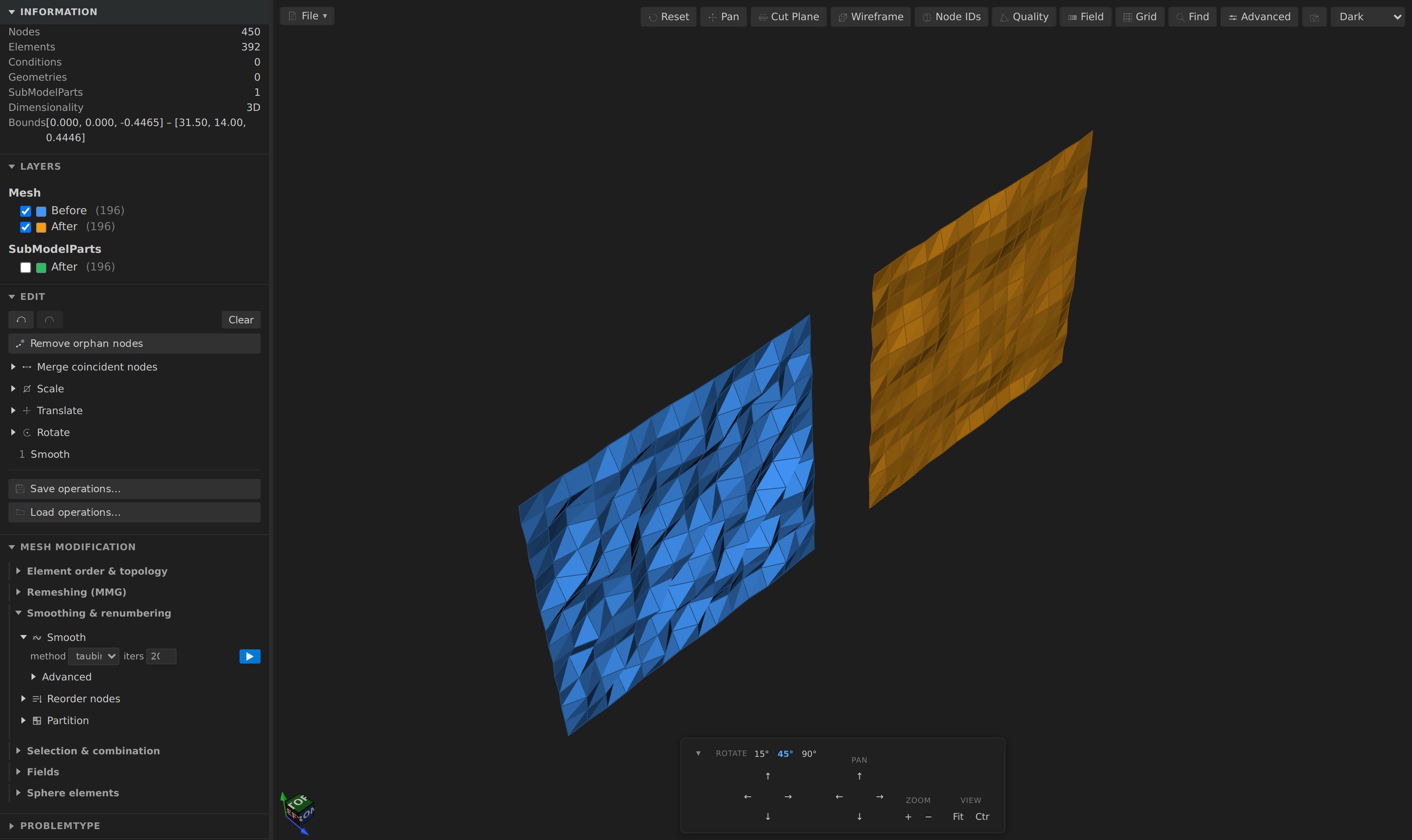
Taubin (the default — it alternates a shrink and an anti-shrink pass, so a closed surface keeps its volume) or Laplacian mesh smoothing. Boundary nodes and sharp-feature edges are pinned by default, and a move that would invert a cell is rejected by default (guard inversion). Only coordinates change — node count, connectivity, SubModelParts and every field come through untouched, which is what makes this safe to apply to a mesh you have already set a case up on.

A third method, ODT (optimal-Delaunay-triangulation), is aimed at a different goal. Taubin and Laplacian smooth a surface; ODT moves each free interior vertex to the volume-weighted average of its incident tetrahedra's circumcenters, which raises element quality — it is the one to reach for before a solve rather than for appearance. It is tetrahedra-only, and says so by name rather than quietly doing nothing if the mesh contains anything else.

Shrinkwrap

Projects the mesh's nodes onto a target triangle surface — a scan, a CAD shell, a coarse solve's boundary — through meshio++'s shrinkwrap. The target is named one of three ways: a file, a SubModelPart of this same mesh, or the mesh's own exterior skin. Each node moves once: x' = x + blend × (p + offset·n − x), with p the closest point on the target and n the normal there (at an edge or vertex, the feature's pseudonormal, so an offset stays on the rounded offset surface). This is a projection, not an iterative or collision-free fit.

• offset stands off along the normal (negative goes to the other side). A target that is not closed has no consistent "outside", so a non-zero offset near its defects can land on different sides — the message says so.
• max dist leaves nodes farther than this in place and counts them; blend is unclamped, so above 1 it overshoots and 0.5 goes half way.
• move only restricts movement to one SubModelPart (and its subtree); keep fixed holds another's nodes exactly where they are (bit-identical, not merely close).
• write distance field adds SHRINKWRAP_DISTANCE, each node's distance to the target before the move, undefined where a node was not queried.

Only coordinates change: blocks, ids, SubModelParts, Properties and every field survive untouched. Because there is no inversion guard, the result message counts the volume cells inverted and surface cells folded over by the move, so a bad projection is reported instead of found by the solver.

Sobolev deformation

Moves the nodes by a raw displacement field after smoothing it through the mesh's own finite-element operators — (M + ℓ²K) u = M d, a screened-Poisson low-pass filter whose cutoff wavelength is the length scale ℓ. It is what turns a jagged per-node displacement (a shape gradient, scattered measurements, a model's raw output) into one a mesh can follow without tangling; short wavelengths are suppressed, long ones pass nearly untouched, and a length scale of 0 applies the displacement unfiltered. Unlike Smooth, which improves a mesh's shape and knows nothing about a field, this filters a displacement you already have and then applies it.

Pick a 2- or 3-component nodal field as the displacement. pin part holds a SubModelPart's nodes exactly in place and pin boundary pins every node on a boundary face; nothing is pinned by default, so an unpinned boundary is free and a constant displacement is preserved exactly, in zero iterations. The mesh's top dimension must be linear lines, triangles or tetrahedra — quads, hexahedra and quadratic cells are refused by name, pointing at Simplexify or Quadratic → Linear. If the iteration cap is reached first, the last iterate is kept and the message says the solve did not converge (raise the cap or lower the length scale); a node the field does not cover moves by 0 and is counted, and the message reports any cell the move inverted.

Reorder

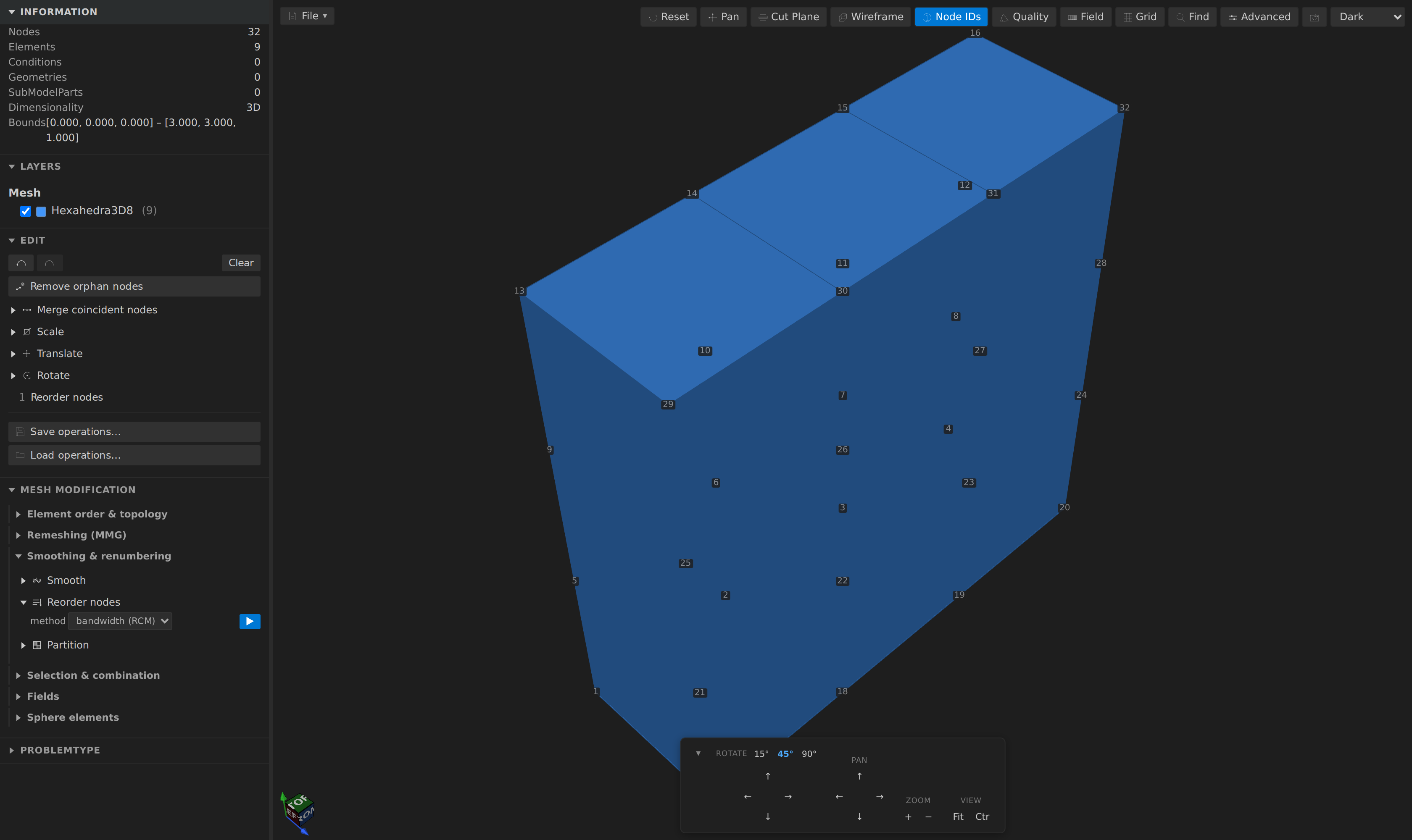
Reorders nodes for RCM bandwidth reduction, or along a Morton / Hilbert space-filling curve for cache locality. This is the one operation with nothing to see in the geometry — it is a pure permutation, so the shot turns Node IDs on, since the ordering is precisely what changed. The coordinates, the cells, the SubModelParts and the fields are all the same mesh, just reordered; the payoff is in how a solver's sparse matrix assembles.

What changes is storage order — which node is written first, second, third — and not the ids: every node keeps its own id and its own coordinates. That is exactly why the SubModelParts and fields come through untouched, since they refer to entities by id and never by position. If you want the ids themselves to change, that is Renumber, below, and running Reorder then Renumber gives you a full RCM renumbering.

Renumber

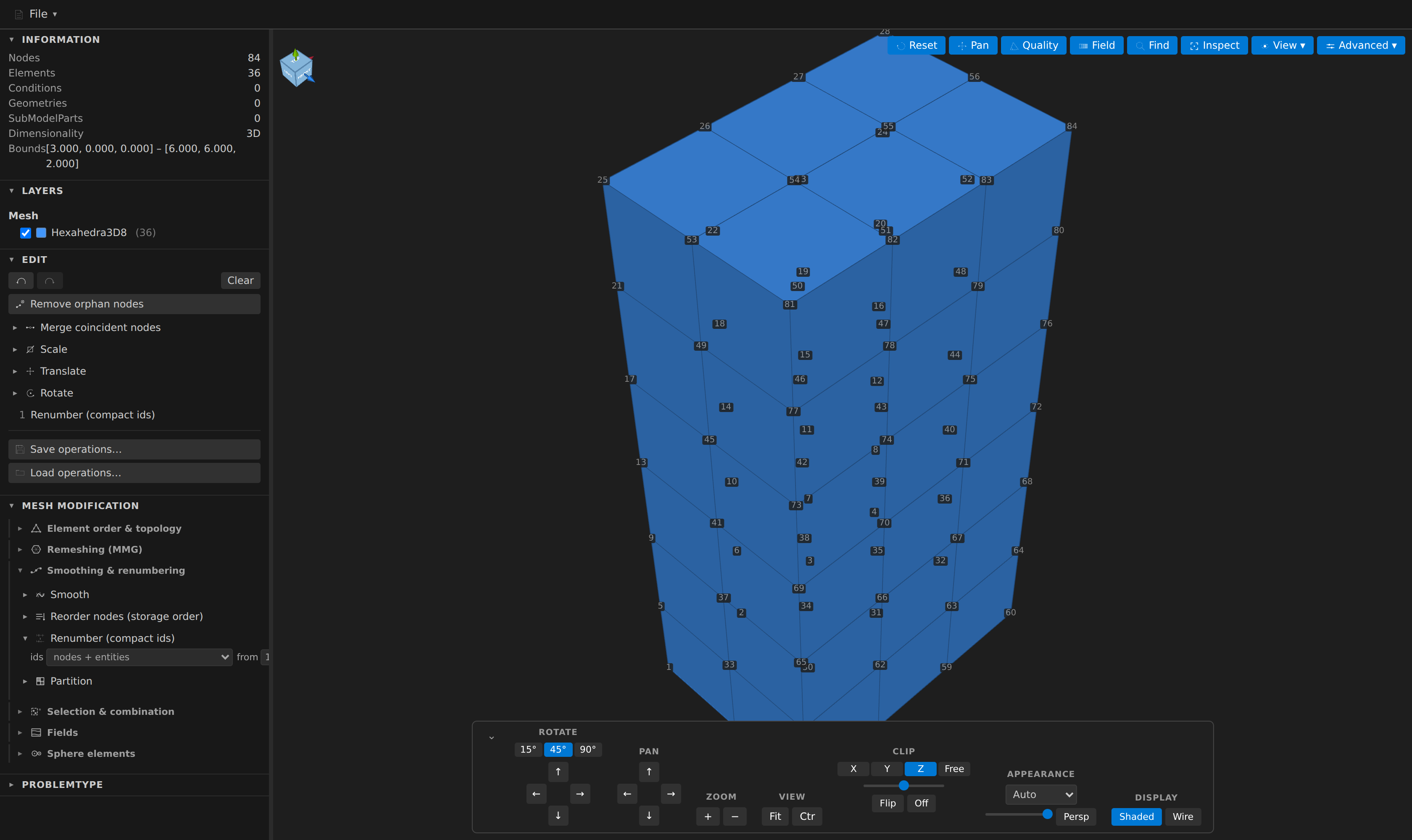
Compacts ids into a gapless run starting at 1, in the order the mesh already stores them. It is the natural cleanup after a Crop, a Merge mesh or a Remove orphan nodes, each of which leaves holes behind: node 5, node 11, node 40 becomes node 1, node 2, node 3, with connectivity, SubModelPart membership and every field record following their ids automatically.

Elements, Conditions and Geometries are each numbered independently, which is what Kratos means — a mesh with Element 1 and Condition 1 side by side is correct, not a collision. You can scope the operation to just the nodes or just the entities, and start the run somewhere other than 1.

Constraints are renumbered too — they are a fourth id space, and a constraint's master and slave node columns follow the nodes just as connectivity does. A constraint whose node did not survive is dropped rather than left pointing at nothing, and the operation says how many went.

Two things are deliberately left alone, because renumbering them would be a guess rather than a relabelling:

• Coordinates. Renumber changes labels, Reorder changes positions.
• Property ids on cells — those index the Properties blocks, a separate id space with its own values (parsed and reported, but never relabelled by this operation).

Constraint ids are also left where they are in the two cases where following them would do harm: when the file lists constraint ids but declares no Begin Constraints block defining them, and when a constraint row is in a shape this extension could not read. Both are reported rather than passed over.

Partition

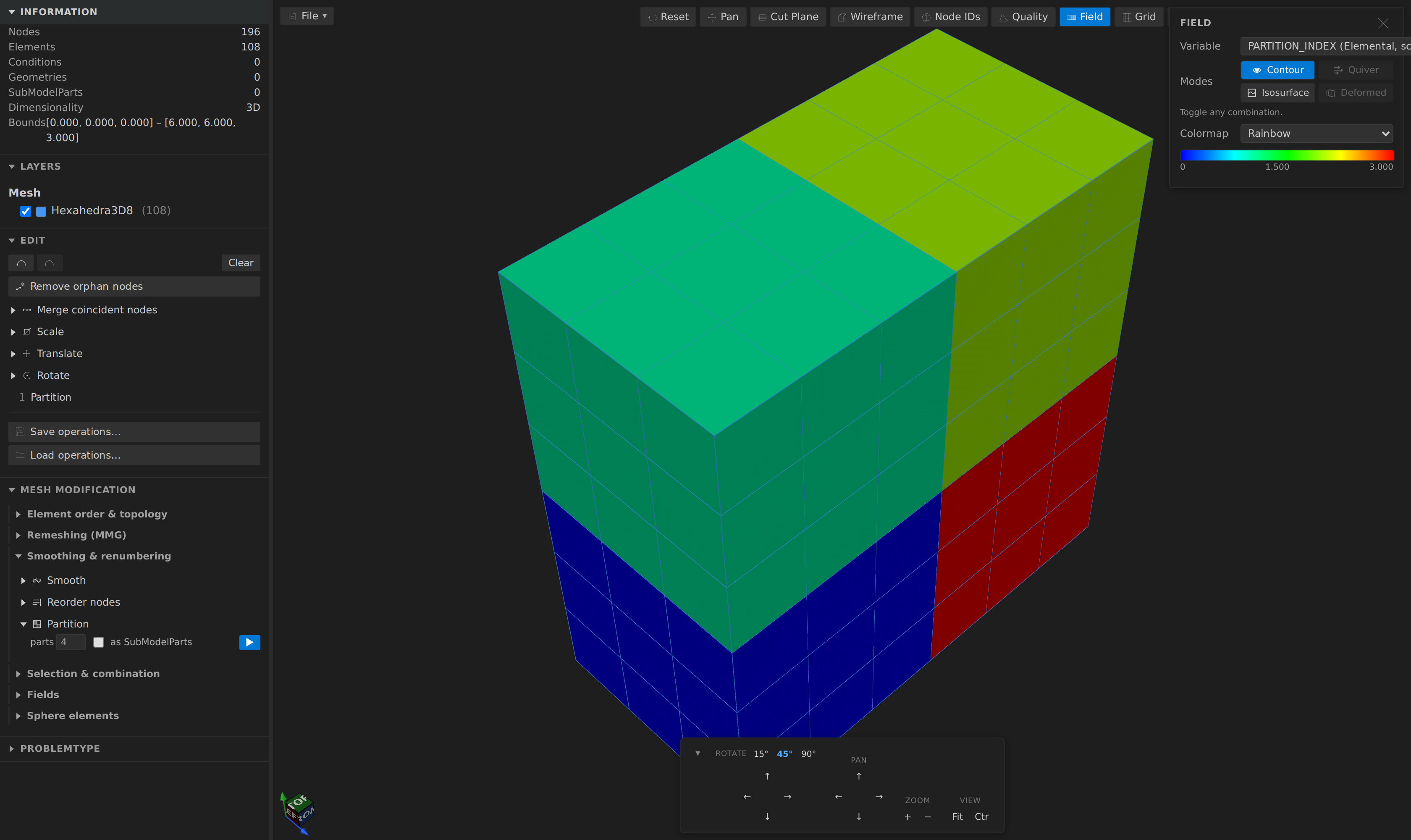
Space-filling-curve domain decomposition into N parts balanced by cell count, attached as a real Kratos PARTITION_INDEX Elemental field (so it exports, and Kratos can read it) and optionally also created as one SubModelPart per part. Colouring by that field through the Field panel is how you check the result, as above. The bundled WASM build has no KaHIP, so only the space-filling-curve method is offered — good for previewing a decomposition and for a quick run, but it minimizes no edge cut and is not a substitute for METIS.

Mark connected components

Writes each Element's connected-component index as an Elemental field (COMPONENT_INDEX, 0 = the largest body, ties broken deterministically): elements sharing a node are connected, and Conditions do not connect bodies, so two bodies a contact condition reaches across are still two. A single body is a no-op that says so. The message lists the elements per component, flags isolated fragments — components under a fraction (default 1%) of the largest, which are usually debris rather than bodies — and counts loose nodes no element uses. Colour by the field to see the bodies, then Split mesh to write each one out. Reachable as the markComponents op.

Selection & combination

Crop

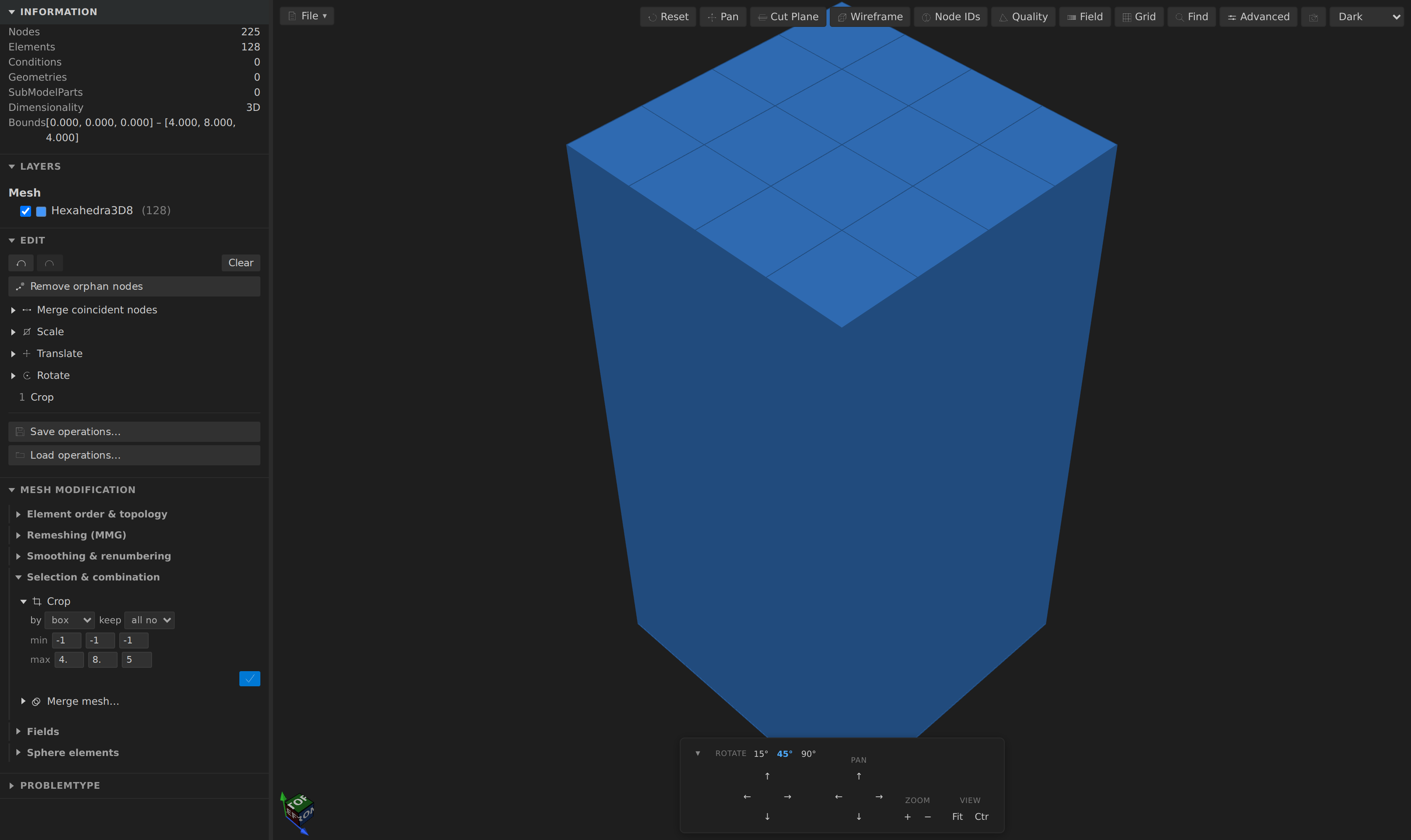
Keeps only the cells inside a bounding box or on one side of a plane, either requiring all of a cell's nodes to qualify or any one of them; anything left unreferenced afterwards is removed. SubModelParts narrow to the survivors rather than disappearing. Above, a box cutting at x = 4.5 keeps half the block.

Merge mesh

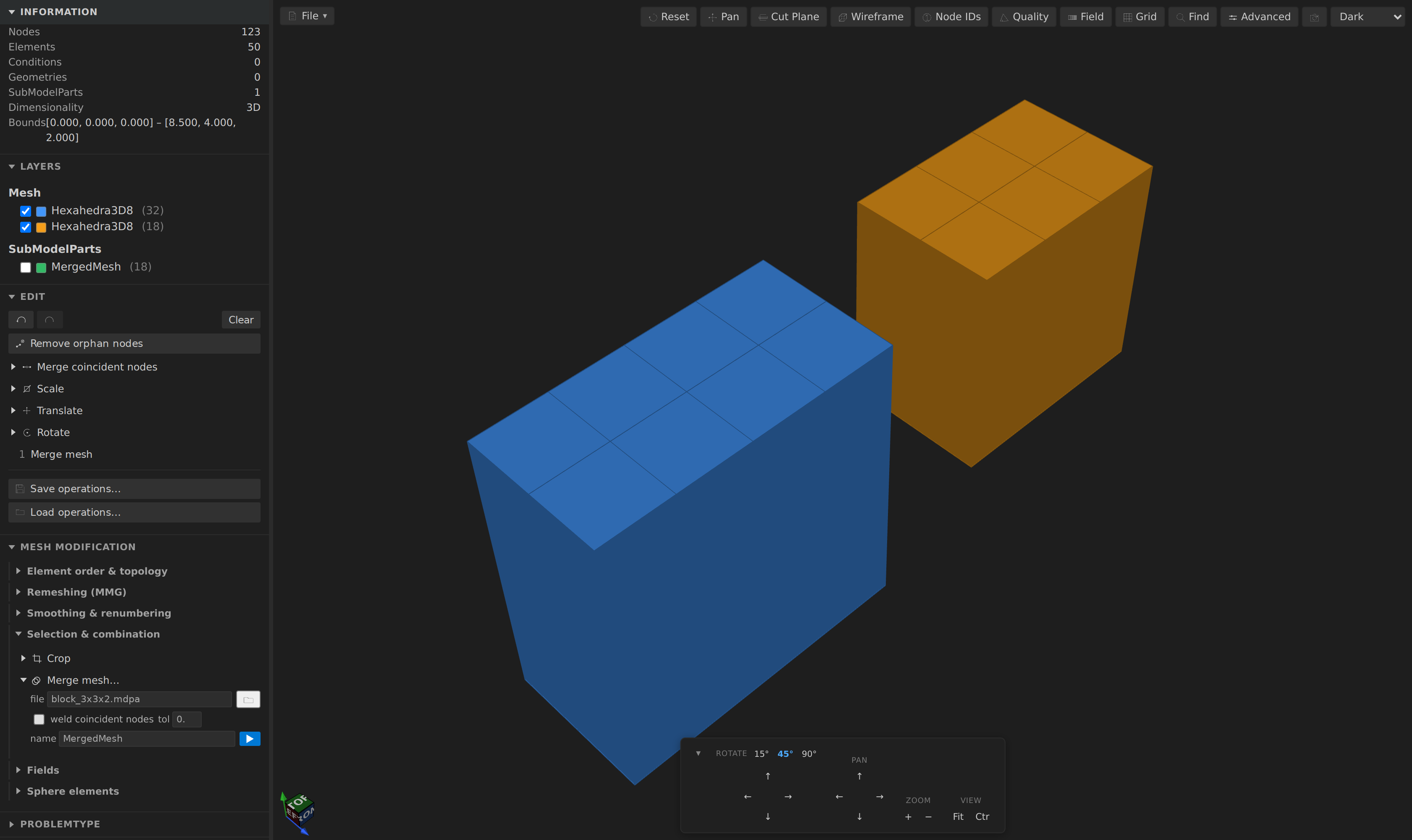
Appends one or several mesh files' nodes and cells, offsetting their ids past the current mesh's maxima and wrapping each merged-in file in its own SubModelPart so you can still tell the pieces apart — frame one, export it or delete it from the outline like any other part. Optionally welds coincident nodes across the seams, using the same tolerance grid as Merge coincident nodes.

Pick several files in the Browse dialog and they merge in one operation: one pass of id offsetting, one weld across every seam, and one entry in the history to undo. Each part is named after its file (beam, column, …), with a _2 suffix if that name is already taken; fill in name and it becomes the parent instead, with the files as its children.

Ids are offset per kind, so elements continue the element run and conditions the condition run rather than both jumping past a shared maximum. That leaves the smallest gaps possible, and Renumber closes what remains.

Two things deserve a warning on merge, and the operation says so rather than leaving you to find out later. A merged file's Properties sets come with it — rebased past your mesh's own Properties ids when they collide, with the merged cells rewritten to follow — so cells that arrive referring to property 7 keep their own property 7 unless yours already has one, in which case they take the next free id and the message names the move. Only a property id the merged file does not define itself is left to resolve against your mesh's Properties. And a field that exists on both sides under the same name but with a different number of components is skipped rather than merged, since one variable cannot be a scalar and a vector at once.

Fields

Field calculator

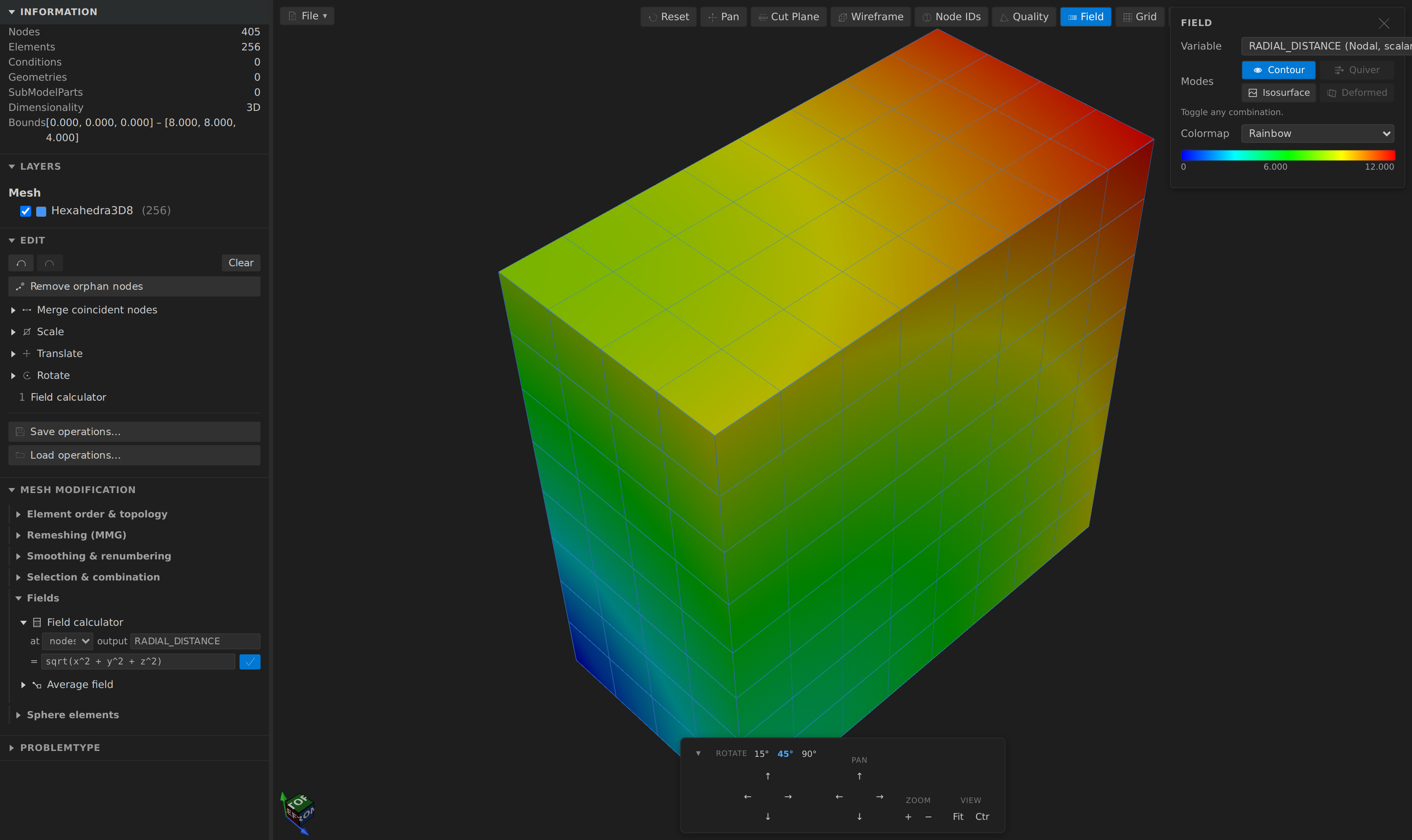
Derives a new nodal/elemental/conditional field from a formula over the node or cell-centroid coordinates (x, y, z) and any existing field at that location — a vector field's components are reachable as NAME_X/NAME_Y/ NAME_Z. It uses the same safe recursive-descent evaluator as the MMG size = ƒ(h) remesh mode, never eval, which matters because a formula can arrive from a saved recipe or a problem archive. A bad formula is rejected inline before anything is applied; a value that cannot be computed (a referenced field is silent at that entity) drops that row, while a genuine infinity from e.g. 1/0 is kept.

Average field

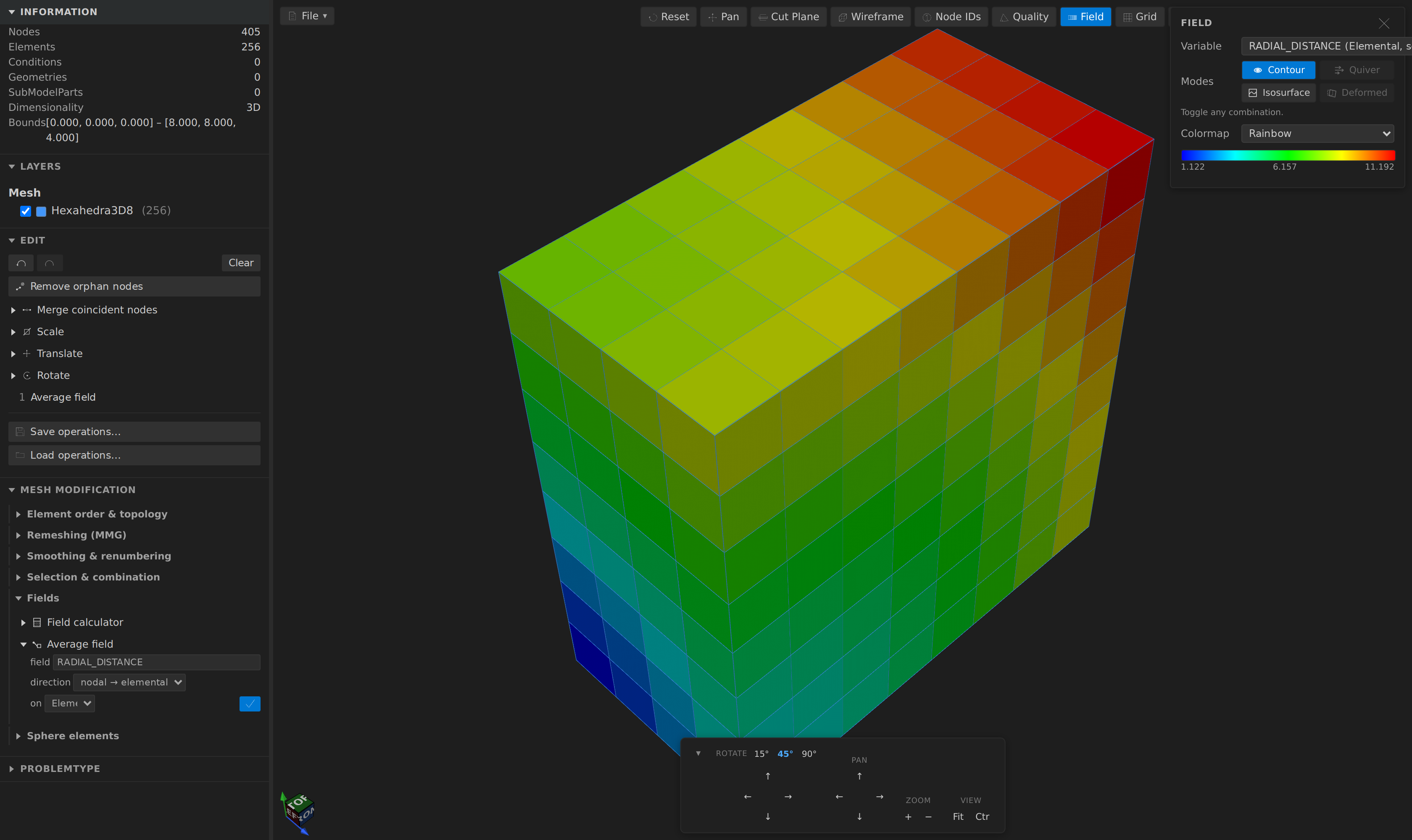
Moves a field between the nodal and elemental/conditional locations by averaging: nodal → elemental takes the mean over a cell's own nodes, elemental → nodal the mean over a node's incident cells (unweighted, not measure-weighted). Above it turns the nodal RADIAL_DISTANCE from the field calculator into a per-element one — note the flat, per-cell colouring against the smooth nodal gradient in the previous shot.

Manage fields

Renames, drops or narrows the fields the mesh carries. Rename keeps the values, ids and nodal fixity under a new Kratos-legal name, refuses a name already taken at that location unless you tick overwrite, and re-points any global reduction that reads the renamed field. Drop removes the selected field; Keep only removes every other field at that location. All three are native and lossless — a field covering only part of the mesh keeps exactly the ids it had — and reachable from mesh_transform as renameField, dropFields and keepFields.

Condition field

Rewrites a field's values without touching its geometry. clamp is min(max(x, lo), hi); normalize maps the field's own [min, max] onto [lo, hi]; standardize gives zero mean and unit (population) standard deviation. Statistics use the finite values only. Scope component conditions each column on its own statistics; magnitude computes them over each row's length and rescales whole rows, so a velocity keeps its direction. NaN decides what a non-finite value does: ignore leaves it and excludes it from the statistics, replace writes a value of your choice, fail refuses the operation. A constant field normalizes to lo and standardizes to 0, and the result message says so. Leave output blank to overwrite in place, or name a field to keep the original beside it. The semantics are those of meshio++'s dataCondition; the implementation is native so a partly-covered field stays partly covered, and fieldManage.test.ts cross-checks it against the live kernel.

A field with more than three components — a Hessian, a stress tensor — now offers every column in the Field panel's Component selector, labelled by index exactly as the data table names its columns (H_0 … H_8), with the row-major position shown for a 3×3 or 2×2 tensor.

Field gradient

Differentiates a nodal field, attaching the result as a new nodal field named <FIELD>_<OPERATOR> unless you name it yourself. The operator picks between the gradient, the divergence and the curl; the latter two need a 2- or 3-component (vector) field. A scalar's gradient has three components and a 3-vector's has nine, laid out as [component][derivative].

The method is a genuine choice rather than a tuning knob. Green-Gauss integrates over each cell's own faces and is exact for a linear field on any cell, which makes it the right default. Least-squares fits over the node-sharing neighbours instead and is smoother on an irregular mesh, falling back to Green-Gauss where a neighbourhood is degenerate.

Two things are reported rather than hidden, because a field that is quietly part-NaN looks perfectly healthy in the field picker: how many cells could not be differentiated at all (a cell below the mesh's own topological dimension, or a degenerate one — these come back NaN, never an approximation), and how many least-squares neighbourhoods fell back.

An elemental field is piecewise constant, so it has no derivative; run Average field in the elemental → nodal direction first and differentiate the result.

Surface curvature

Measures the discrete curvature of a surface mesh (triangles and quadrilaterals) at every node, through meshio++'s computeCurvature, and writes it as ordinary nodal fields: CURVATURE_MEAN (H), CURVATURE_GAUSSIAN (K) and, on request, CURVATURE_K1/CURVATURE_K2 (the principal curvatures, k1 ≥ k2, as two scalar fields) and CURVATURE_AREA (the dual area the curvatures were divided by). A sphere of radius R reads H = 1/R and K = 1/R². Dual area picks between mixed-voronoi (exact on a well-shaped triangulation) and barycentric (more forgiving of obtuse triangles); boundary nodes asks for the nodes of an open surface, which otherwise have no curvature and are left as gaps — never 0.

Two things are reported rather than left to mislead. The sign of the mean curvature follows the winding, so a surface wound inside-out reads −1/R; when neighbouring faces disagree the message says the sign is unreliable and points at Repair surface. And for a closed surface the message includes the Gauss–Bonnet check: the sum of the angle defects against 2πχ (4π for a sphere), which is a mesh-independent way to see that the numbers are sound. A solid is refused by name — measure its skin (File ▸ Export skin…) instead.

The fields are usable anywhere a nodal field is: colour by them in the Field panel, or size a remesh with them. The Curvature-adaptive surface preset in the Remesh (MMG) size = ƒ(h) mode is clamp(0.3/max(abs(curvature_mean), 0.000001), 0.5*min, 1.5*max) — about twenty elements per full turn of the local radius of curvature, bounded to half the smallest and one and a half times the largest current element — and computes CURVATURE_MEAN first when the mesh has none. mesh_curvature returns the same statistics headlessly without writing any field.

Field Hessian

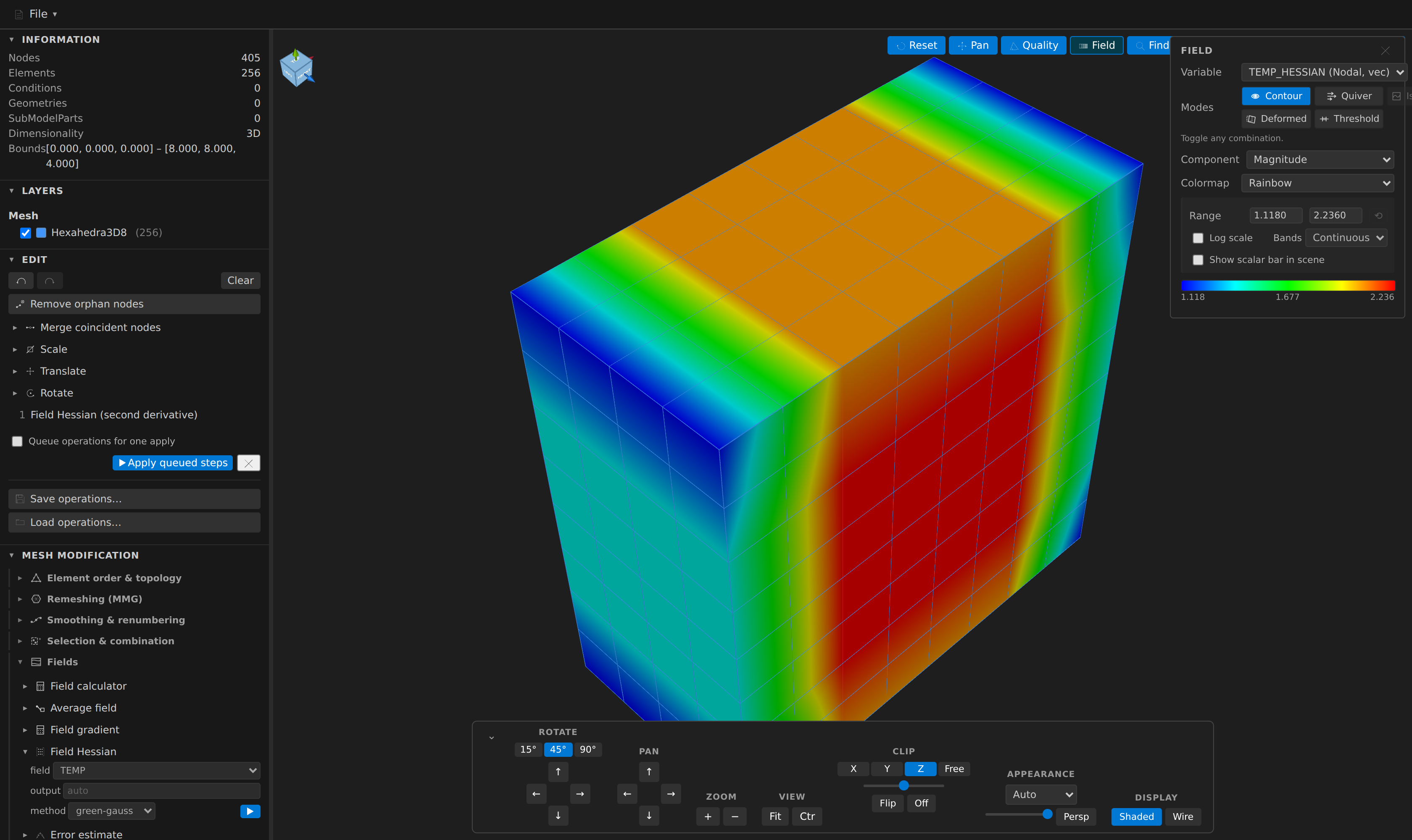
The second derivative of a scalar nodal field, attached as a new nodal field of nine components — the flattened row-major 3×3 matrix, with H[i][j] at index i*3+j. It is Field gradient's companion one order further, and the two share the same method choice, forwarded to both internal passes.

The guarantee worth knowing is what it says about your mesh rather than about the operation: a field that is at most linear has an exactly zero Hessian everywhere, on any mesh. That is the one shape-independent property, so a linear field coming back non-zero is a red flag. For a genuinely curved field the result is exact on a structured mesh away from its own boundary and a good, standard, but genuinely approximate curvature estimate on an irregular one — it is a composition of two gradient passes, not a separate numerical kernel.

The Hessian is defined for one component at a time, so a vector field is refused rather than silently reduced: split it with the field calculator and run this once per component. An elemental field is refused for the same reason Field gradient refuses one, with the same fix.

Error estimate

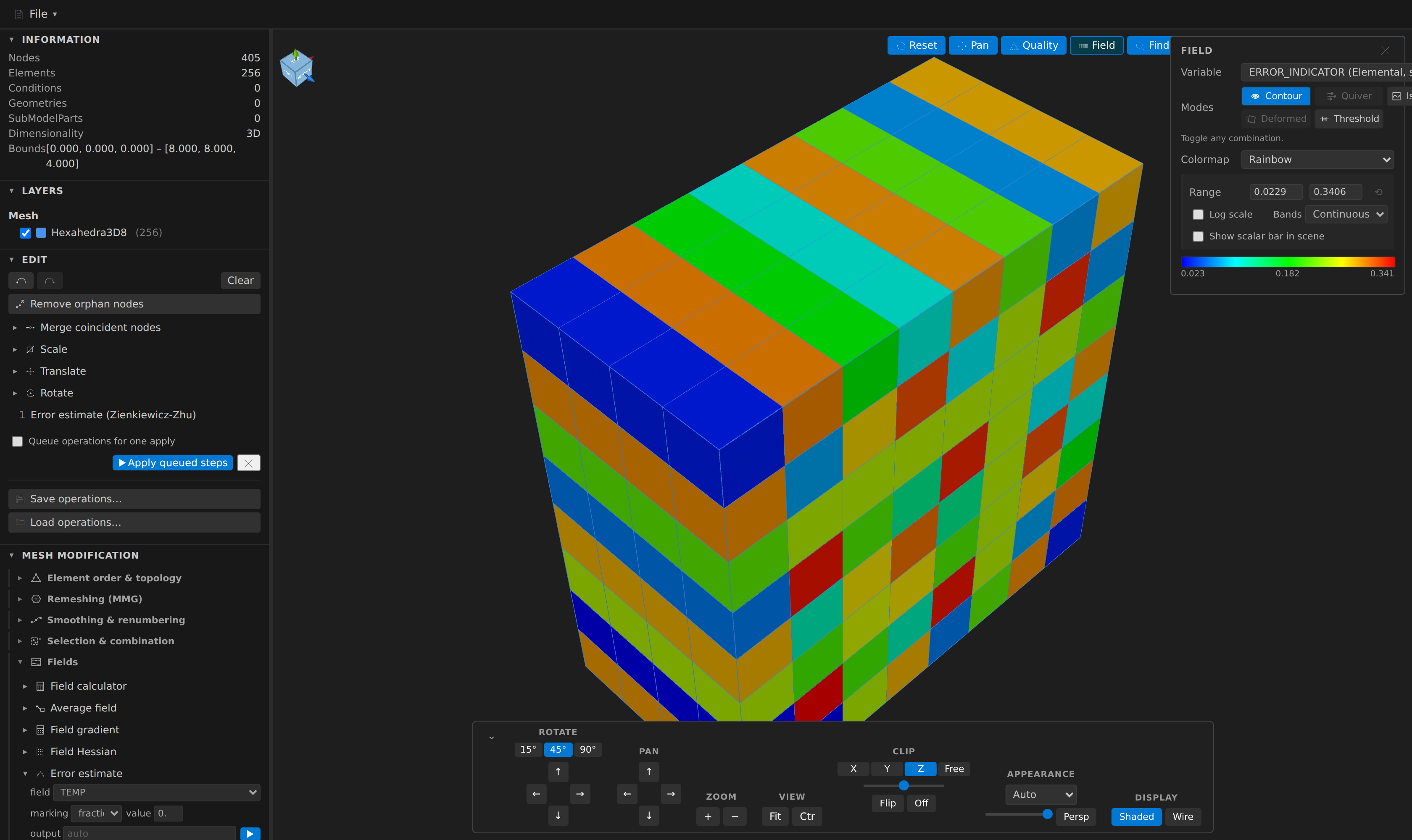
Answers "where is this mesh not good enough for this solution?" using the Zienkiewicz–Zhu recovery-based indicator: per cell, sqrt(measure × Σ(recovered − raw gradient)²), attached as an Elemental field (ERROR_INDICATOR by default).

Read a near-zero result as good news, not a failure. The estimator compares a smoothed gradient against the piecewise one, and for a field the mesh represents exactly — anything linear — those agree, so the error genuinely is zero. A curved field on a coarse mesh is where the numbers appear.

Marking turns the indicator into an actionable 0/1 flag in a second ERROR_MARKED field: absolute thresholds the indicator directly, fraction marks that share of cells worst-first, and dörfler marks the smallest set of cells holding that share of the total error. Because it is an ordinary field, the Field panel's threshold mode will isolate the marked cells for you, and it rides a .mdpa export like any other elemental data.

Cells that cannot be evaluated read NaN in the indicator but 0, never NaN, in the marking array — so a marking field is always safe to threshold on. The count is reported alongside the global error.

Distance to surface

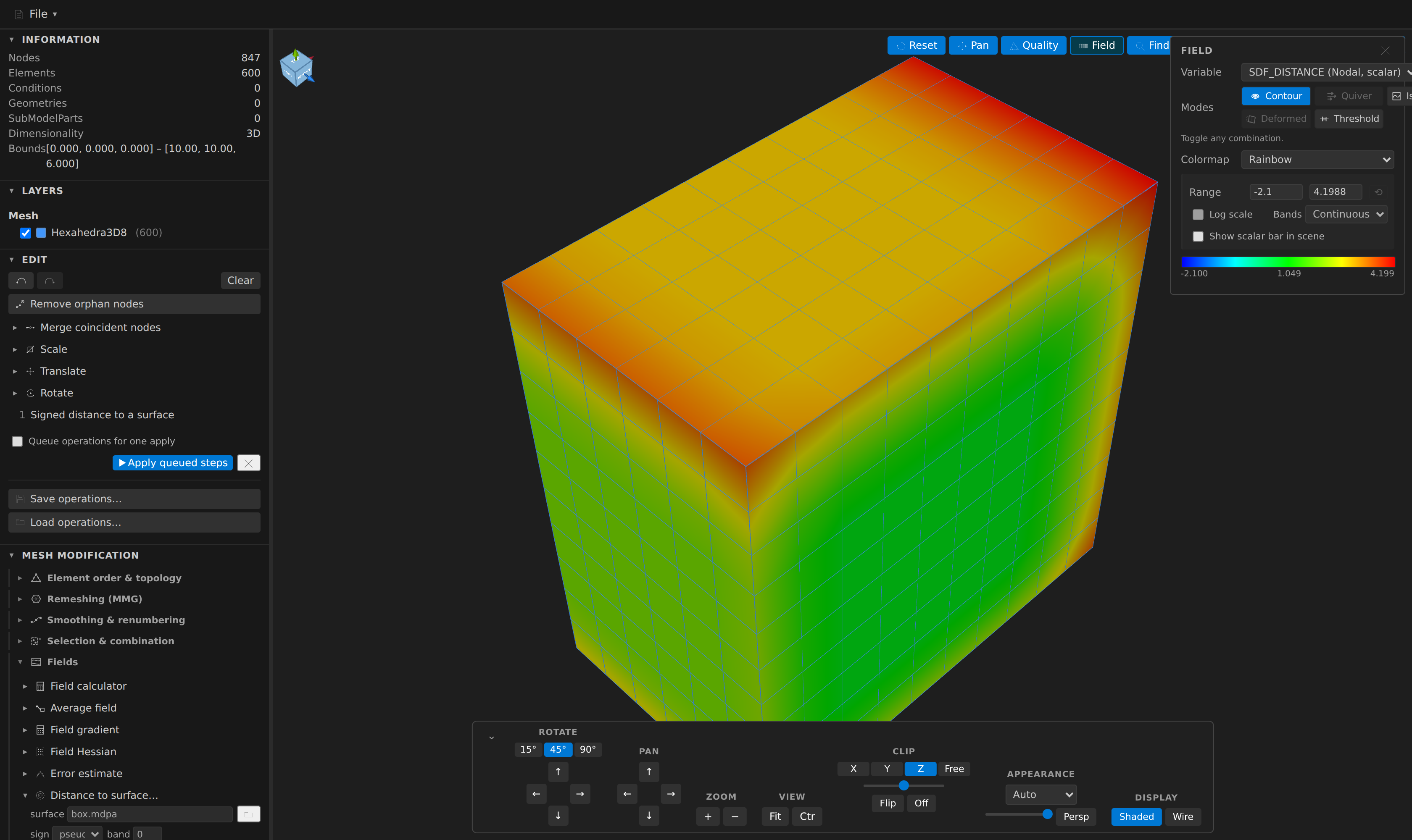
Measures the signed distance from every node of this mesh to a surface mesh you pick from disk, as a new nodal field (SDF_DISTANCE by default). Negative is inside. The surface needs triangle cells: an edge-only boundary (e.g. a 2D wall part) is refused with a message rather than a cryptic backend error.

The pairing is the point: Level-set split (MMG) already cuts a mesh along the isosurface of a nodal field, but there was no way to get such a field from an imported geometry. Run Distance to surface, then Level-set split on its output, and you have cut your mesh along that surface — no new machinery, two ordinary undoable operations.

The sign mode decides how inside/outside is determined. Pseudonormal is the fast angle-weighted test and the right default; winding uses the generalized winding number, slower but tolerant of small holes; unsigned skips the question entirely, which is what you want for an open surface, where "inside" has no meaning. Band trades accuracy for speed by computing exact values only within a given distance of the surface and clamping beyond it.

Compare with another mesh

Compares one of this mesh's fields with the same field of another file and writes the difference, so "how far did this run drift from that one" becomes something you can colour by. Three fields are written under the chosen name (default: the field's own): <name>_DIFF (signed a − b, same width as the field), <name>_ABS (the Euclidean norm of the difference) and <name>_REL (relative to |b|, left as a gap where |b| is 0). The result message gives how many entities were compared, max |a−b| with the id where it occurs, the RMS and mean, the largest relative error and, when you set atol / rtol, how many rows fall outside |a−b| ≤ atol + rtol·|b|.

• by id reads the same entity id from the other file — nodes by node id, elements and conditions each in their own id space — so it needs the two meshes to share an id space (a re-run, an edit, a restart). It is order-free.
• spatial point-samples the other mesh's nodal field at this mesh's nodes (barycentric, through meshio++'s interpolate), for two different discretizations of the same domain. It is deliberately not Transfer fields: that one conserves totals and smooths nodal data through a cell round trip, this one samples. A node outside the other mesh — or whose sampling cell touches a node with no value — is uncovered: counted, and a gap in the output, never 0. For a surface mesh a point counts as covered when it projects inside a cell; its distance off the surface is not checked. A cell field cannot be sampled this way — move it to the nodes with Average field first.

Entities with no counterpart, and non-finite values, are gaps in every case. For the structural comparison — a verdict, moved nodes with the worst id, entities only in one mesh or with changed connectivity (node order is the winding, so a rotated node list counts), renamed blocks, SubModelPart membership differences and per-field norms — use the mesh_compare MCP tool; it compares the models themselves rather than a lossy conversion, which is why it can see ids, kinds and SubModelParts that meshio++'s diff never does.

Transfer fields

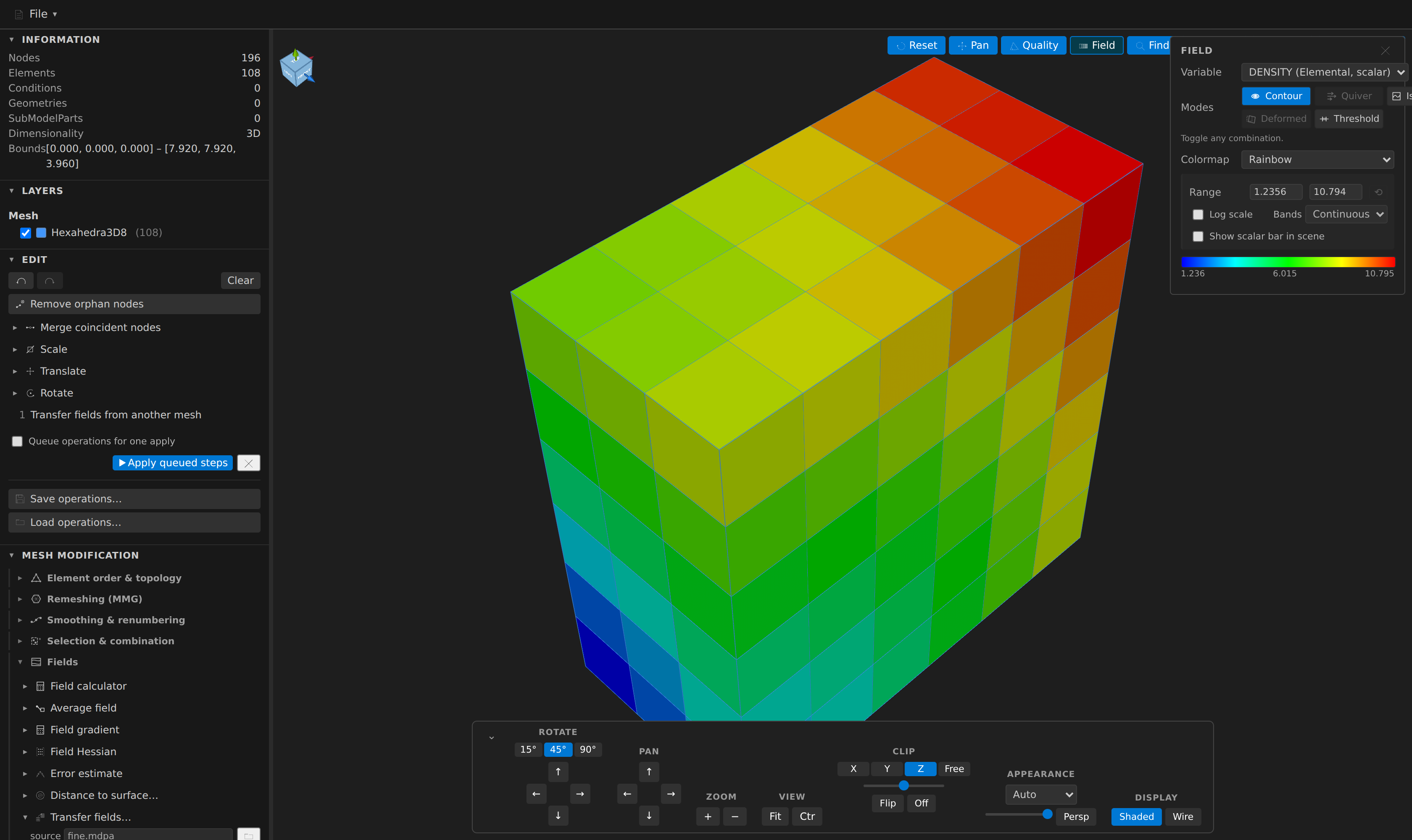
Maps another mesh's fields onto this one — mapping a coarse solution onto a refined mesh, or bringing a solver result back onto the geometry you are editing. It uses conservative interpolation: over the region the two meshes share, the measure-weighted sum is equal on both sides. For anything that is a density — mass, energy, a source term — pointwise sampling quietly changes the total, and the total is usually what mattered.

Two consequences are worth stating up front:

• Nodal data is smoothed, not resampled. The conservation guarantee is cell-based, so nodal fields travel by a point → cell → clip → point round trip. A constant field survives exactly; a varying one comes back averaged, even between two identical meshes. This op is for moving data between different discretizations, not for copying a field you already have.
• A field that no longer fits is dropped, and named. Both meshes are simplexified internally (a hexahedron fans into six tetrahedra), so a transferred cell array can come back with a different entity count than this mesh has. Rather than scatter values onto the wrong elements, such an array is discarded with a diagnostic naming it.

Leave fields empty to transfer everything the source carries. On clash decides what happens to a name that already exists here: overwrite (the default, so re-running updates), suffix, or error.

Variables

The Variables sidebar section is the named registry over all of the above: every field on the mesh — parsed from the file, computed by any of these forms, mapped across a remesh, or made headlessly — has a row here, so this panel and the Field panel (which lists the same inventory, badging row-claimed fields with a ● and a reveal jump) can never disagree about what exists.

Add a variable by hand (+ Add variable), name it (e.g. d), and pick how to compute it: a formula over coordinates and existing fields at any location (Nodal/Elemental/Conditional, the same locations the Field calculator offers), the signed distance to a surface (an imported file, or a SubModelPart already in this mesh; the same sign/band options the Signed-distance form offers), any other operation from this section (average, gradient, Hessian, error estimate, transfer — the same options as their forms, each with its form's icon), or a global reduction (min/max/minAbs/maxAbs/mean/std/median/sum/count/q1/q3/iqr of any field, e.g. maxAbs_TEMP; vectors reduce over magnitude). Computing a field from any of the forms above instead creates the row for you, prefilled with that form's inputs. Once computed it is an ordinary field — the Field panel opens on it automatically — and it is immediately usable anywhere else a formula is accepted, notably the MMG size = ƒ(h) remesh formula, so a d computed here can drive a boundary-layer grading like clamp(0.85*mean_h*(abs(d)/maxabs_d), 0.85*min_h, 1.15*max_h) with no separate wiring. Picking that Boundary-layer preset goes one step further: whatever it needs and the mesh doesn't have yet (d, plus mean_h/min_h/max_h globals of the mesh size and a maxabs_d global — the largest |d|) is added here automatically, and everything needing no further input is computed at once — d's surface stays your call, and so does pressing Play on maxabs_d once d exists (it reads d, which cannot be computed before then). A global is a single number rather than a field: its row shows the live value, and it is usable in every formula by name (a global can never go stale — its value is recomputed from the current fields wherever it is used).

Fields with no reconstructible definition (file fields and the like) render as locked rows — name, kind and origin, show-on-mesh, delete — and deleting any row removes only the row, never the field. A row tracks the field it produced: if the field vanishes (e.g. a time-series step replays without the async op that computed it), a definition row says so and offers recompute instead of keeping a stale "Computed.", while a tracking row simply leaves with it.

Reorganizing the SubModelPart tree

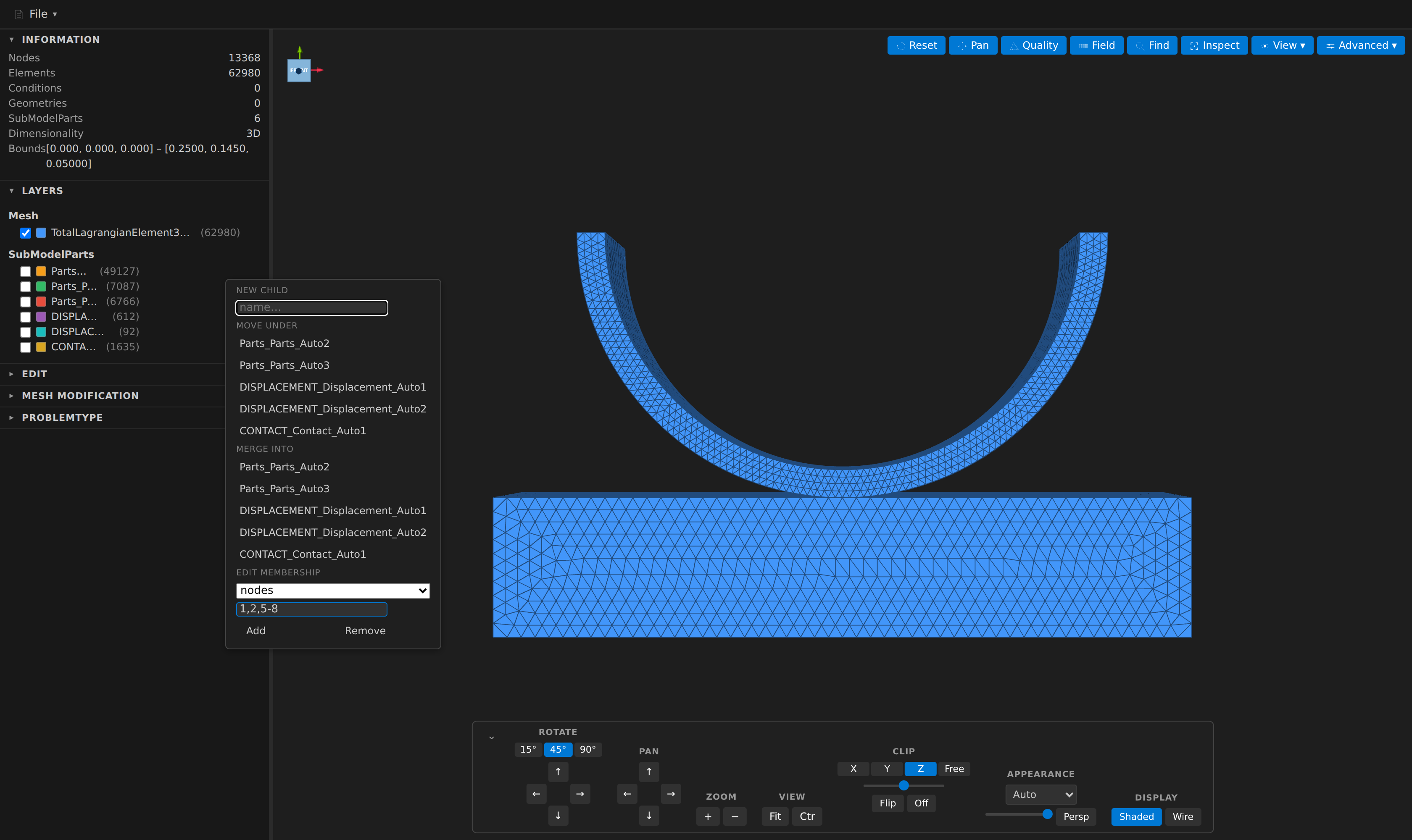
Every SubModelPart row in the outline carries an organize button beside the rename and delete ones. It opens a small menu with four things:

• New child — type a name and press Enter to create an empty SubModelPart under this one. (Names follow the same rules as rename: non-empty, no /, and no clash with an existing sibling.)
• Move under — reparent this part anywhere else in the tree, or back to the top level. Every descendant path is rebased with it.
• Merge into — fold this part into another: the target gains the union of the entity ids, this part's children re-attach under the target, and this part disappears.
• Edit membership — add or remove node, element, condition or geometry ids directly: pick the kind, type a comma-separated id list with optional ranges (1,2,5-10), and press Add or Remove. Removing changes membership only — the node or element itself stays in the mesh, just no longer claimed by this part.

Destinations that cannot work — the part itself, or anything inside its own subtree — are simply not offered.

The parent/child rule is maintained, not just checked

Kratos requires a child SubModelPart's entities to be a subset of its parent's. Rather than refusing operations that would break that, these operations keep it true the same way Kratos itself does: adding an entity to a part also adds it to every ancestor, and removing one also removes it from every descendant — which is precisely what ModelPart::AddNode and ModelPart::RemoveNode do upstream. Moving and merging propagate upward for the same reason. Whenever that touches parts you did not name, the operation's message says how many ids moved, so nothing happens silently.

Adding and removing entity ids directly is available as the mesh_transform ops addSubModelPartEntities / removeSubModelPartEntities (and in a saved recipe). Note that removing an entity from a part only changes membership — the node or element itself stays in the mesh.

Simplify surface

Advanced ▸ Simplify surface… (or Kratos Mesh: Simplify Surface) writes a simplified copy of a triangle surface through meshio++'s quadric-error edge collapse — an export, never an edit, because decimation is lossy by intent. It asks what percentage of the faces to keep; the mesh_derive tool (kind: "decimate") also takes an absolute targetFaces, or a maxError (collapse only while the cheapest candidate's quadric error is at most this, in squared mesh units), with the placement of the surviving vertex (optimal, midpoint, endpoint).

• Boundary and creases stay put. Boundary vertices are pinned, so an open patch keeps its outline exactly, and vertices on creases (dihedral above 30°) are pinned so a cube keeps its corners; a frozen SubModelPart pins more. If pinning leaves no collapsible edge before the target is reached the run stops there and says so.
• Survivors are the source's own faces. A collapse removes one or two faces and leaves every other face in place with one corner redirected, so a surviving face keeps its entity id, kind, block name, property id and every elemental/conditional field value — never averaged. A node keeps the lowest id merged into it, at the placed position; its nodal fields are upstream's blend of the collapsed endpoints (exact for midpoint/endpoint, an approximation for optimal). SubModelParts are narrowed to survivors; constraints are dropped with a stated warning, since the topology changed.
• The report states the cost. Faces and nodes before and after, the achieved reduction, and the largest collapse error — also as a share of the bounding-box diagonal, which reads the same at any scale.
• What it refuses, by name: volume cells (use Export skin first), quads (Simplexify first), higher-order cells (Quadratic → Linear first), and lines or points mixed into the surface (their nodes would dangle after a collapse).

View ▸ Level of detail is the preview counterpart: it draws a decimated surface in place of the full layers so a very large mesh stays navigable. The mesh, its history, its saves and its exports are untouched, and the layers are suppressed rather than hidden, so their visibility comes back exactly as it was. A solid is drawn by its boundary skin. Because a decimated triangle is a re-meshed patch that no source cell owns, picking is off while it shows and the status line says so.

Sample to grid

Advanced ▸ Sample to grid… (or Kratos Mesh: Sample to Grid) writes the surface — or, for a solid, its boundary skin — sampled on a regular lattice. It is an export: the open mesh is never changed and nothing lands in the history.

• Voxel occupancy writes the cells whose centre is inside the surface (a VOXEL_OCCUPANCY field of 1s). The MCP tool can also write the cells a triangle passes through (fill: "surface") or the whole box (fill: "all").
• Signed-distance volume writes the distance from every lattice point to the surface, negative inside, as the nodal field SDF_DISTANCE, padded by a tenth of the bounding-box diagonal so the zero level is well inside the lattice. sign: "winding-number" tolerates small holes; "unsigned" drops the sign. An octree (adaptive, with hanging nodes) is available through MCP and is never a dense lattice.
• The cost is stated first. The cell size you enter gives nx × ny × nz cells, points and an approximate memory figure before anything is allocated; above five million cells the extension asks for confirmation, and anything over twenty million is refused outright.
• .vti is offered only when it is true. An unstructured model cannot reconstruct a structured lattice, so .vti is written straight from meshio++'s own mesh and only for a complete lattice (an SDF volume, a whole-box voxelization or a plain grid). A partial voxelization or an octree is refused as .vti by name and writes as .vtu (or any other cell format) instead. The .vti keeps the sdf:* header that no other format carries.
• What it refuses, by name: a mesh with no surface faces (lines or points only); an open surface is sampled but the message warns that the sign is unreliable near the holes — repair it first, or use the winding-number sign.

Export partitions

Advanced ▸ Export partitions… (or Kratos Mesh: Export Partitions) writes the mesh as N per-part files plus a <stem>.partitions.json manifest — the file-per-rank layout a distributed run starts from. It asks for the number of parts, the number of ghost layers (face-adjacent neighbours each part also holds; 0 for none), a folder and a format, and refuses to overwrite silently.

• Every cell is owned by exactly one part. meshio++ decides ownership and, with ghost layers, which neighbours each part also holds; every part is then rebuilt natively from the source cell ids, so ids, Elements/Conditions/Geometries kinds, Properties, SubModelParts, fields and (when every node they name survives) constraints all carry over. A part is a Kratos mesh, not a meshio++ conversion, and because ids are preserved the "original-id map" is the identity — the manifest says idsPreserved instead of shipping million-entry arrays.
• Ghosts are distinguishable. Each part carries PARTITION_INDEX (the owner of every cell — a ghost's is its neighbour), PARTITION_GHOST (0/1) and a Ghost SubModelPart holding the ghost cells and the nodes only they use.
• The manifest gives, per file, the owned and ghost counts by kind, the node count and the interface nodes (owned nodes shared with another part — what a solver exchanges over), plus the imbalance (max/mean owned elements − 1).
• Weights (MCP only): weights names an Elemental field of per-element weights, so a region that costs more is spread over more parts.

The WebAssembly build has no KaHIP: kahip is refused by name and the method is a Hilbert space-filling-curve cut — balanced by cell count (or weight), with good locality, but no edge-cut minimization. mesh_capabilities reports which partitioners the live build can actually run. This produces partitioned data; solver-specific distributed Kratos setup is a separate matter.

Split mesh

Advanced ▸ Split mesh… writes one file per connected body, per element type, or per distinct value of a scalar elemental field (up to 1000), with a <stem>.split.json manifest. Like the partition export it keeps the source's ids and everything attached to them. A Condition that names nodes of two different bodies belongs to neither and is counted in the manifest rather than silently attached to one; isolated fragments are flagged. Both exports are reachable together as the mesh_split MCP tool.

Export skin

Advanced ▸ Export skin… is not an in-place edit but an export: it extracts the boundary of the mesh's volume cells (plus any pre-existing surface cells) as a standalone surface mesh and writes it to a file of your choice, through the same format picker as File ▸ Export. It is a native boundary-face walk — a face seen by exactly one cell is boundary — rather than meshio++'s own surface/skin extractors, so SubModelParts survive the extraction (narrowed to node membership; element/condition membership cannot follow, since the skin's faces get fresh entity ids). Also reachable from the mesh_extract_skin MCP tool.

Edit operations

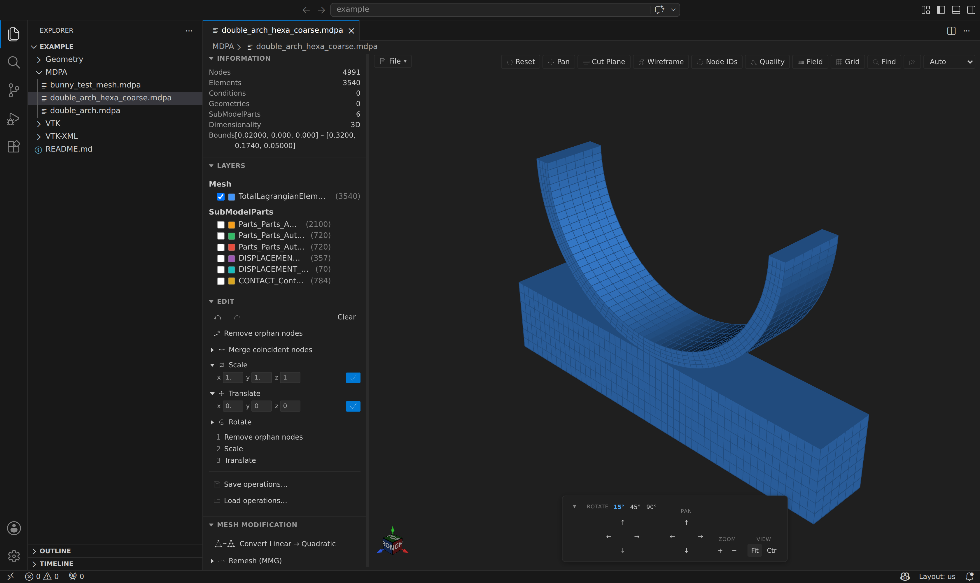
The Edit section hosts interactive, form-driven operations — enter the values inline and press Apply (or Enter in a field):

• Remove orphan nodes — drop nodes referenced by no cell and listed in no SubModelPart.
• Merge coincident nodes — weld nodes within a tolerance into one.
• Scale — per-axis scale factors (x, y, z).
• Translate — offset by (dx, dy, dz).
• Rotate — by an angle in degrees about the X, Y, or Z axis, through a configurable center point (defaults to the origin).
• Delete a SubModelPart — triggered from the ✕ button on a SubModelPart row in the outline tree; its entities and any orphaned nodes are removed.
• Set element radius — set or scale the RADIUS of one-node (sphere/particle) elements, optionally limited to one SubModelPart. See Sphere / Particle Elements.

Each transform form is a collapsible dropdown — click its title to expand its inputs.

Operation history

Every applied edit — including Linear → Quadratic and the MMG operations — is recorded in the history:

• Undo / Redo / Clear controls.
• A clickable list of the applied operations. Clicking an entry partially reverts the mesh to that step; later steps stay redoable until you apply a new operation.

Because the operations are pure and deterministic, the history is a replayable recipe:

• Save operations… writes the applied operations to a JSON file.
• Load operations… replays a recipe onto the current mesh.

Ctrl+Z and Ctrl+Shift+Z undo and redo without leaving the viewport, and work wherever the focus is inside the preview. They are the same undo the sidebar buttons drive, so the two never disagree. From the Command Palette they are Kratos Mesh: Undo Mesh Operation / Redo Mesh Operation.

Unsaved edits and the dirty marker

Applying an operation marks the preview tab unsaved — the dot in the tab, the same one a modified text file gets. Closing it asks before discarding, and a window that closes with edits still pending brings them back when it reopens (VS Code's hot exit; what is stored is the operation recipe, not a copy of the mesh).

Two details are worth knowing, because both are deliberate:

• The marker is a latch. It clears when you save the mesh, or on File ▸ Revert File — which drops every operation and re-reads the file from disk. Undoing your way back to zero operations does not clear it: the preview would rather ask once too often than let real work disappear. The Edit section's Clear button does not clear it either, for the same reason.
• Saving must actually write to clear it. If the save is refused — an OpenFOAM case, a format with no writer, or you dismiss the overwrite confirmation — the tab stays marked and nothing is written.
• A preview never auto-saves. If you use files.autoSave, it does not apply here: saving a preview re-serialises the whole mesh over the source file, and the overwrite warning is only shown once, so an automatic save would quietly rewrite the file you opened one second after your first operation. Automatic saves are refused and the tab simply stays marked; Ctrl+S and File ▸ Save work as normal. Set kratos.preview.autoSave to true if you want auto-save to apply anyway.

Scrubbing a VTK time series is not an edit, so stepping through a solver's output never marks anything unsaved.

Two flavours of "Save As"

Kratos Mesh: Save Mesh As… (Ctrl+Shift+S) is the one to use: it keeps the source format, falls back to .vtu when that format has no writer, refuses to rewrite an OpenFOAM case under the preview reading it, and leaves your history intact. VS Code's own File ▸ Save As also works, but — as it does for any editor — it replaces the tab with one for the new file, and the operation history does not come with it.

Combining several operations into one apply

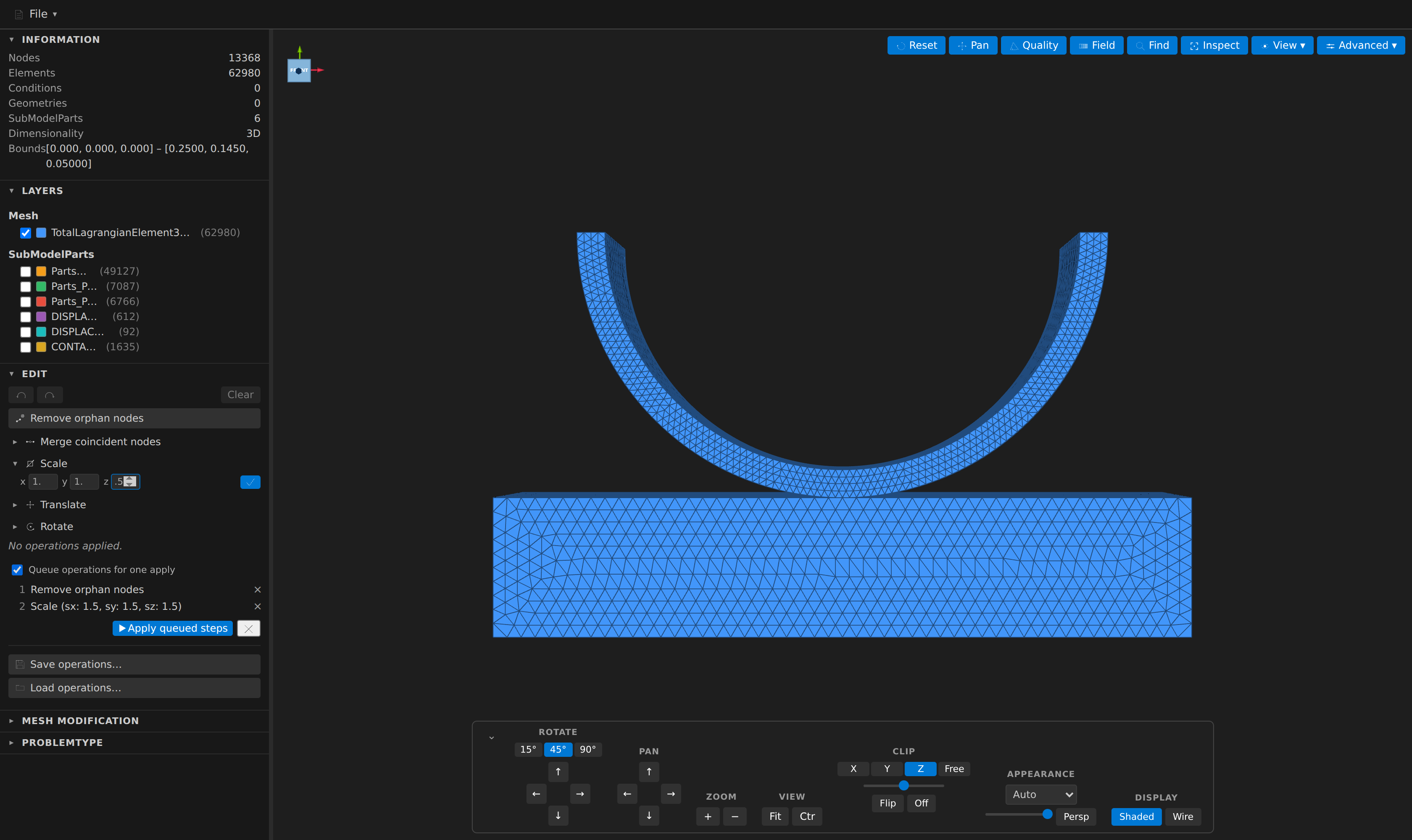
Every sidebar form normally applies the moment you click its Apply button — one click, one history entry, one toast. Check "Queue operations for one apply" (in the Edit section, above Save/Load operations) and that changes: every Apply button across the whole sidebar — Edit's transform forms and every Mesh Modification form — stages its operation into a list instead of running it immediately. Build up as many steps as you like, from as many different forms as you like, in whatever order you click them; each staged row shows a short summary of what it will do and a × to drop it again.

Click Apply queued steps and they run in that order, in one sequence, under one progress bar. Each step still lands as its own ordinary, independently undoable row in the history — queuing only saves you the clicks and the toasts, it does not change how the steps are recorded. Undo peels them off one at a time, same as any other operation.

A queue that hits a stopping point — you cancel it, or a step fails outright — keeps whatever already succeeded. Nothing is rolled back; the toast tells you how far it got, and the mesh reflects exactly the steps that ran.

Reloading, and what happens to your edits

File ▸ Reload from disk (Ctrl+Alt+R, or the Kratos Mesh: Reload from Disk command) re-reads the file. So does an external change to it — the preview watches the file — and, for a .mdpa, saving it in a text editor.

Your edits survive all of that. The history is re-applied to the new contents rather than thrown away, so a colleague regenerating the mesh, or a solver appending a time step, no longer silently costs you an afternoon's work. Two things are worth knowing about how that goes:

• An operation that no longer applies is kept, not dropped. If the file changed such that an op has nothing to do — you deleted a SubModelPart that is already gone — the op stays in the list marked no effect, with its own explanation as the tooltip, and the operations after it still run. Nothing is destroyed, so you can revert to before it or clear it yourself.
• Stepping a VTK time series skips the expensive operations. Geometric ops (scale, crop, refine, delete part, …) follow you from frame to frame, but the remeshing and meshio++-backed ones (MMG remesh, level-set split, smooth, reorder, partition, merge, field gradient) are marked skipped rather than re-run — a 30-second remesh firing on every arrow-key press would make the timeline unusable. Re-apply skipped operations, which appears in the Edit section whenever there is something to re-run, runs them on the current frame.

TIP

The history still belongs to the loaded mesh, so opening a different file starts fresh. Save operations… remains the way to carry a recipe between meshes.