Plot Presets

The Plots quick panel carries a Preset selector that builds a complete, validated plot recipe from a few inputs — no manual source wiring. The same builders back the plot_preset MCP tool, so a preset assembled by hand in the viewer and one built headlessly are the same recipe evaluated by the same worker. Presets never invent data: every parameter they need is supplied, every gap is reported, and every refusal names its reason.

The five presets

Field distribution

A histogram of one component (or the magnitude) of a Nodal, Elemental or Conditional field over the mesh entities, optionally within one SubModelPart, at the current frame. The Field panel's Plot distribution button opens it for the field you are looking at, and the quick panel's Show on mesh does the reverse. Entities the field does not cover are excluded and counted as gaps, never as 0.

Section comparison over time

One curve per SubModelPart for a field's mean over time — inlet against outlet pressure is the canonical case. The operation is the boundary mean by default (the faces owned by exactly one element of the part) or the entity mean; a vector field plots its magnitude or one X/Y/Z component. Supply explicit physical times (one per frame) with a timeUnit and the axis is time; without them it is a step label, honestly rather than by assumption. Differences are deliberately not derived here: read them off the curves or the exported table, or ask for them explicitly (see below). Needs at least two distinct SubModelParts.

Measure-weighted total

The sum of a scalar Elemental field times each element's length, area or volume — a total mass from a density field, a total power from a flux field — per SubModelPart or over the whole mesh. Elements with no value or no measure are excluded and counted, never treated as zero. Over a series it draws one line per region; for the current frame it draws bars.

Tensor and vector components

One curve per component index of a tensor or vector field over time for a SubModelPart — give the component indices or just the field width (plots 0 through width−1). Components are named by index only: the file states no Voigt order, so no stress, strain or invariant meaning is inferred. The mean is over the part's entities by default, or its boundary.

Tensor invariants

Von Mises, hydrostatic (trace/3), trace, J2, deviatoric norm, principal maximum/middle/minimum and maximum shear (half the largest principal difference) of a tensor field over time for a SubModelPart, as the mean (or min/max) over its entities. You supply the component layout; it is never guessed: full3x3 (row-major xx, xy, xz, yx, yy, yz, zx, zy, zz), full2x2, or explicit indices {xx, yy, zz, xy, yz, xz} for a Voigt-style order (e.g. {xx:0, yy:1, zz:2, xy:3, yz:4, xz:5}). Leave out zz/yz/xz for a plane problem — they are taken as zero and the result says so. Choose engineering shear when the off-diagonals are stored as γ = 2ε; they are halved. A row with a non-finite component is a gap, never zero, and a layout that does not fit the field's width is refused by name. Units follow the source field (J2 is a squared unit, so none is claimed).

Heat-flux balance

The flux of a supplied nodal heat-flux vector through boundary SubModelParts over time, positive out of the domain. The field is taken as given — no conductivity or temperature gradient is used or inferred — with the same outward-or-winding orientation choice and optional 2D thickness as the Flow Balance panel.

Table relationship

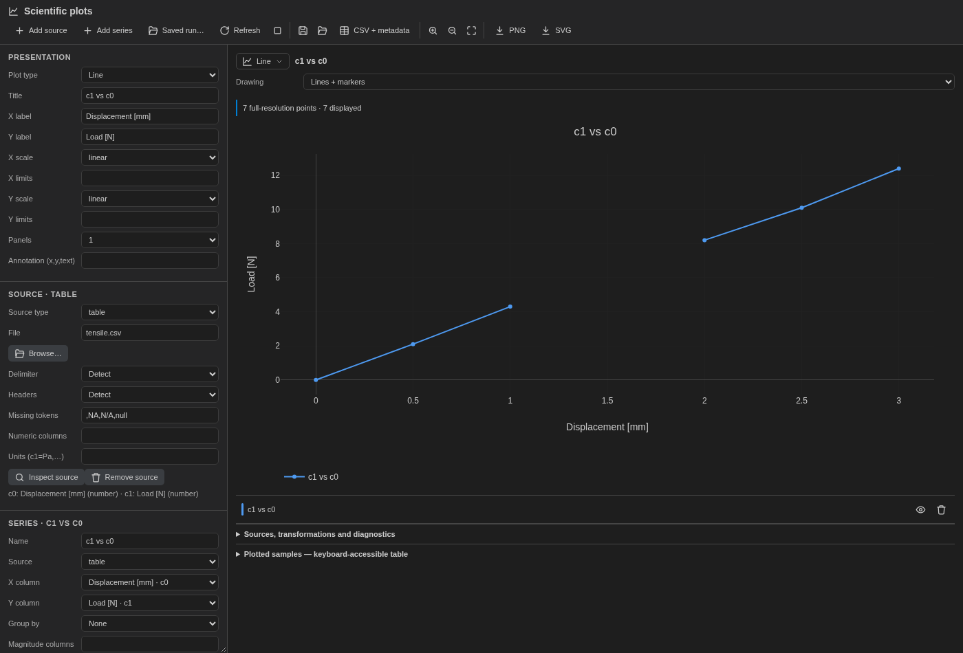
One supplied table column against another — load against displacement, pressure against flow — with x/y as the importer's column ids (c0, c1, … in file order, as plot_table_read shows them) and only the units the table supplies. Line or scatter.

Pressure-density conversion

A boundaryMean or mean region source — and therefore the section-comparison preset and plot_preset — accepts an explicit pressureDensity in kg/m³ for a field that records SI kinematic pressure (m²/s²) and reports it in Pa, so two sections subtract into a genuine pressure drop. The density is never inferred, and anything that is not a kinematic-pressure field under one of those two operations is refused by name. Unknown, already-physical and non-pressure fields stay exactly as they are.

Threshold check

Any evaluated preset run (or any plot_preset call with evaluate) can carry a threshold: a user-supplied limit with a direction, above or below. Equality is not a violation, and a gap is counted apart — never passed, never failed. The answer reports how many points were checked, how many were gaps, how many exceeded, the first and the worst exceedance with its margin, and a single ok. It is a check, not a verdict on the run: it says whether a curve stayed inside a limit you set.

Section differences

With differences: [{from, to}] (series ids), an evaluated run also reports from − to at exactly matching x — the pressure drop between two section curves, for example. An x present on only one side, or a gap on either side, is a gap in the difference, never 0; series whose units differ are refused rather than subtracted. Combined with pressureDensity, two kinematic-pressure sections difference into Pascals.

In the viewer

The quick panel's Preset selector offers the section comparison and the measure-weighted total against the open mesh: it prefills the path, the current field and the SubModelParts, and the built recipe lands in the workspace like any hand-assembled one — editable, exportable, and saved with the same provenance. The remaining presets are reachable through plot_preset today; the panel selector does not yet drive them, which is stated rather than hidden so nobody hunts for a control that is not there.