Laminar flow around an obstacle

A viscous Newtonian fluid (density 1000 kg/m³, dynamic viscosity 0.6 Pa·s) flows at 0.1 m/s past a 120 mm obstacle in a 2.0 × 0.6 m channel. You sketch and mesh the channel, then solve it monolithically in Kratos. At a Reynolds number of 20 the flow stays laminar, with stagnation at the upstream face and a small reversed-flow pocket behind the obstacle.

At a glance

Mesh	945 nodes, 1766 cells
Run	51 frames, end time 5
Kratos packages	KratosFluidDynamicsApplication==10.4.3
Download	fluid case with its verification record

What you will learn

• Build a face with a hole from a sketch, and name the Parts it needs.
• Grade a mesh around a curved boundary, and solve a classic-VMS case with a Bossak time scheme.

The physical model

The Reynolds number, Re = ρUD/μ, is 1000 × 0.1 × 0.12 / 0.6 = 20 for the case values, with 0.12 m the obstacle diameter. At this Reynolds number viscosity dominates and no turbulence model is needed. The turbulent version of the problem is a separate tutorial.

The inlet imposes a uniform 0.1 m/s in +X, and the outlet holds the pressure at zero. The channel walls are slip walls, so the obstacle is the only no-slip surface and the only source of drag and wake.

The case uses the monolithic formulation with the Classic VMS (legacy) element, as the Mok fluid–structure tutorial does on its fluid side. The built-in element default is Quasi-static VMS. The case pins classic VMS with the Bossak time scheme because the BDF2 scheme segfaults this Kratos 10.4.3 build at the first solution step.

Create the geometry

1. Open cad/examples/BREP/blank.brep in CAD mode. Choose File → Import SVG… and open obstacle-channel.svg. It makes a 2000 × 600 mm channel with a 32-segment, 60 mm-radius obstacle at (500, 300) mm.
2. Switch to Line selection, select all 36 edges, and choose GEOMETRY → 2D → Surface → Build. The preview should show one face with one opening.

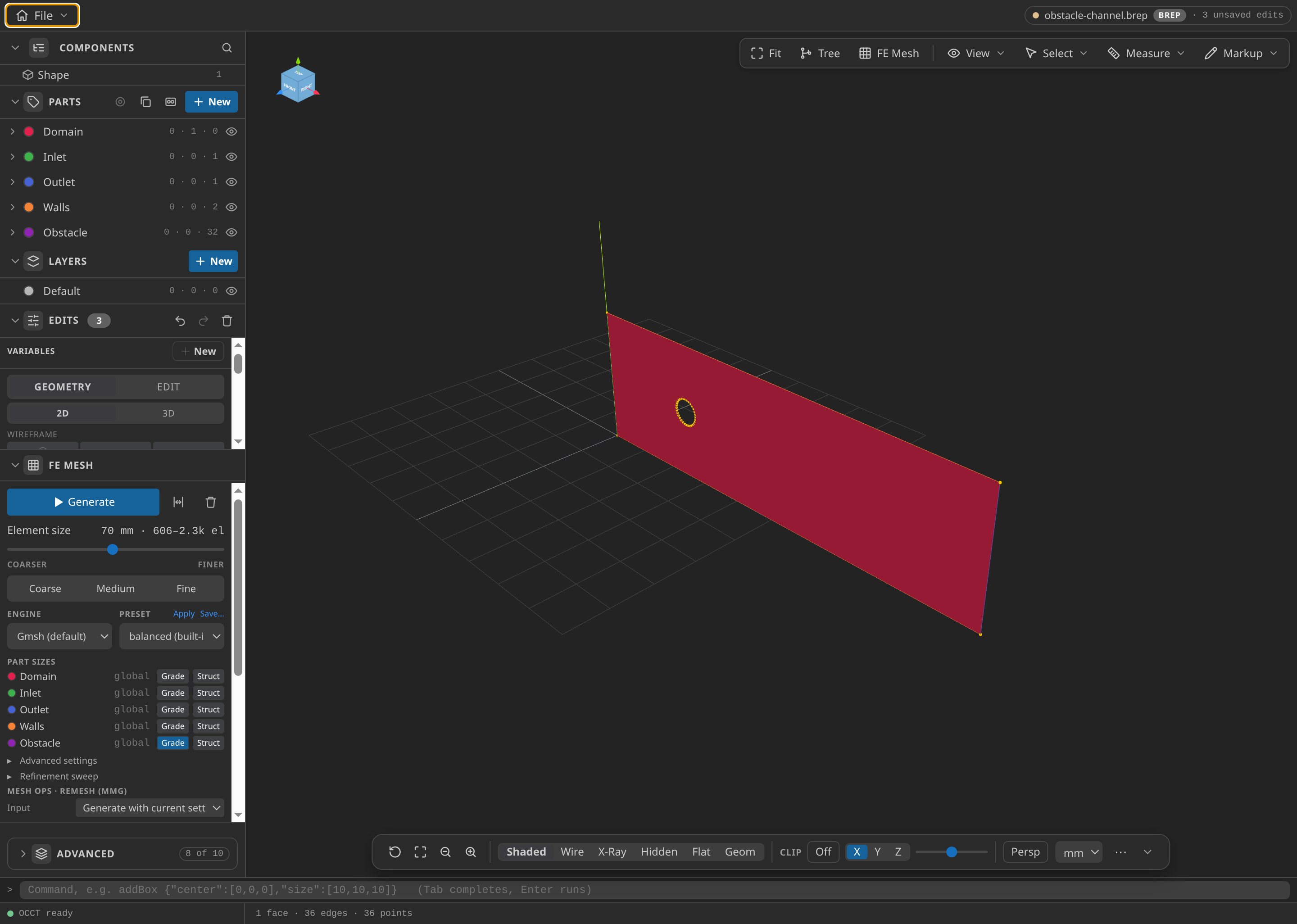
The channel face after Build, with its Parts named.

The obstacle is a 32-sided polygon by design. Gmsh sizes the first row of cells from the boundary edges, and the 11.8 mm chord of 32 sides pins that row whatever the wall size asks for.

Name the Parts

3. Under Parts, name the face Domain; the left edge (x = 0, edge-3) Inlet; the right edge (x = 2000 mm, edge-1) Outlet; the top and bottom edges (edge-0, edge-2) Walls; and the 32 obstacle edges Obstacle.

Each name becomes a SubModelPart that conditions attach to. A Part missing from the mesh is a Preflight error.

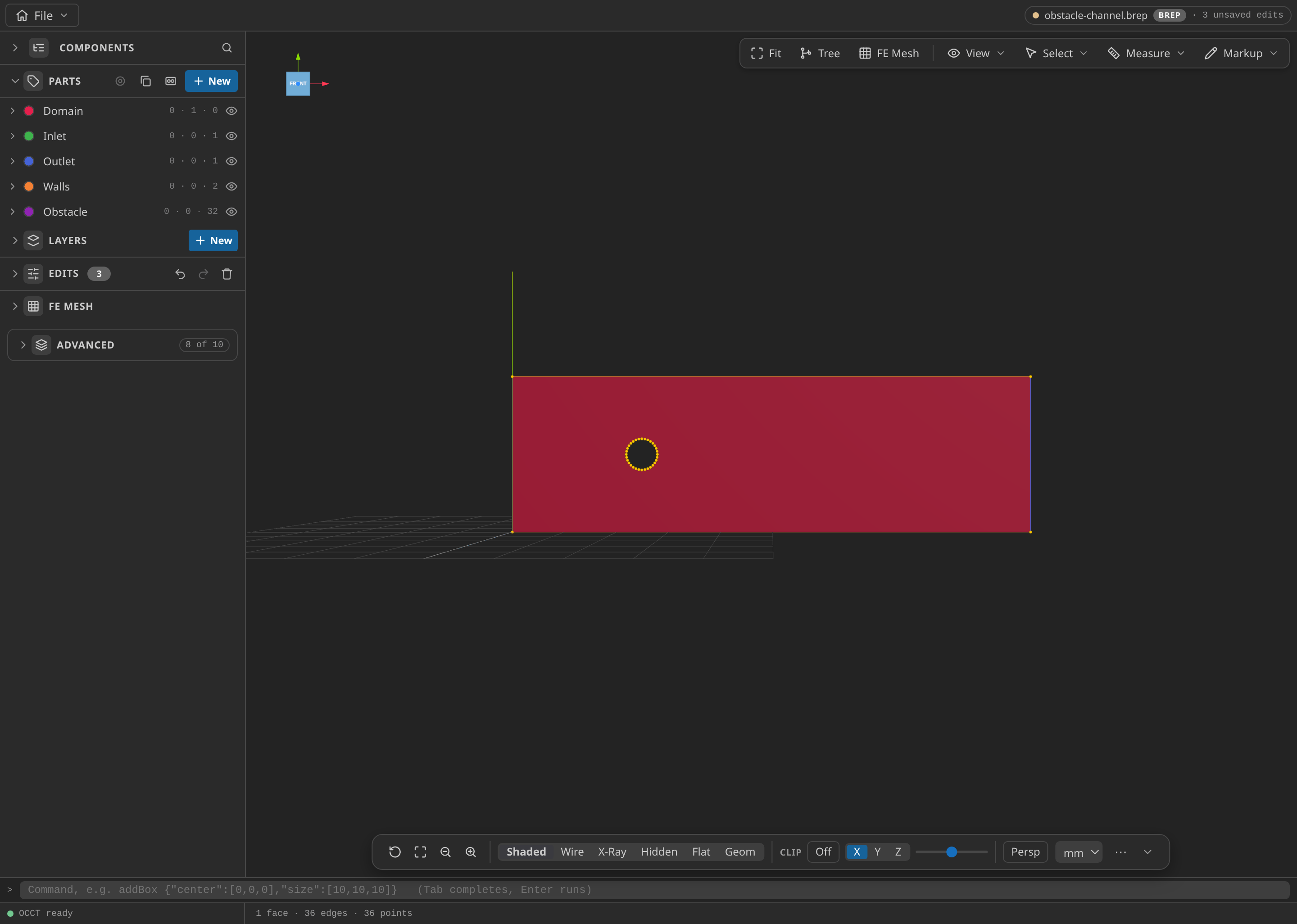
The CAD window with the Parts panel open, showing the named Parts: Domain, Inlet, Outlet, Walls and Obstacle.

Mesh

4. Under FE Mesh, choose Gmsh, 2D, first order, and set the global size min/max to 15/70 mm. In the Obstacle Part's Grade controls, set the size at wall to 12 mm, the size far to 60 mm, the distance near to 25 mm and the distance far to 350 mm. Choose MDPA Elements, export units m, and export as mesh.mdpa.

The grade keeps cells small at the obstacle. The export has 945 nodes and 1766 triangles. That is deliberately modest: the checks test the setup and the physics on this mesh, not a converged answer.

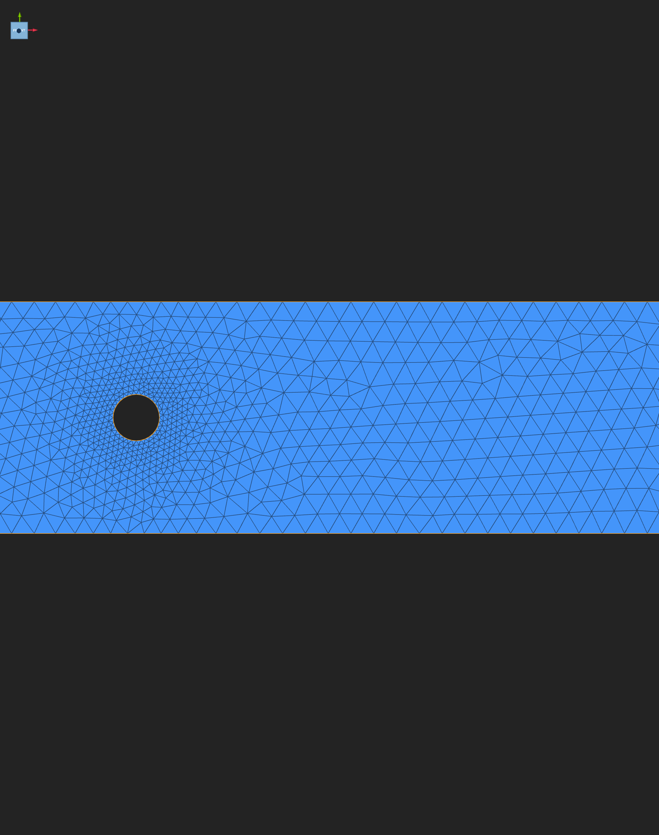
Small triangles hug the obstacle and grow toward the outlet.

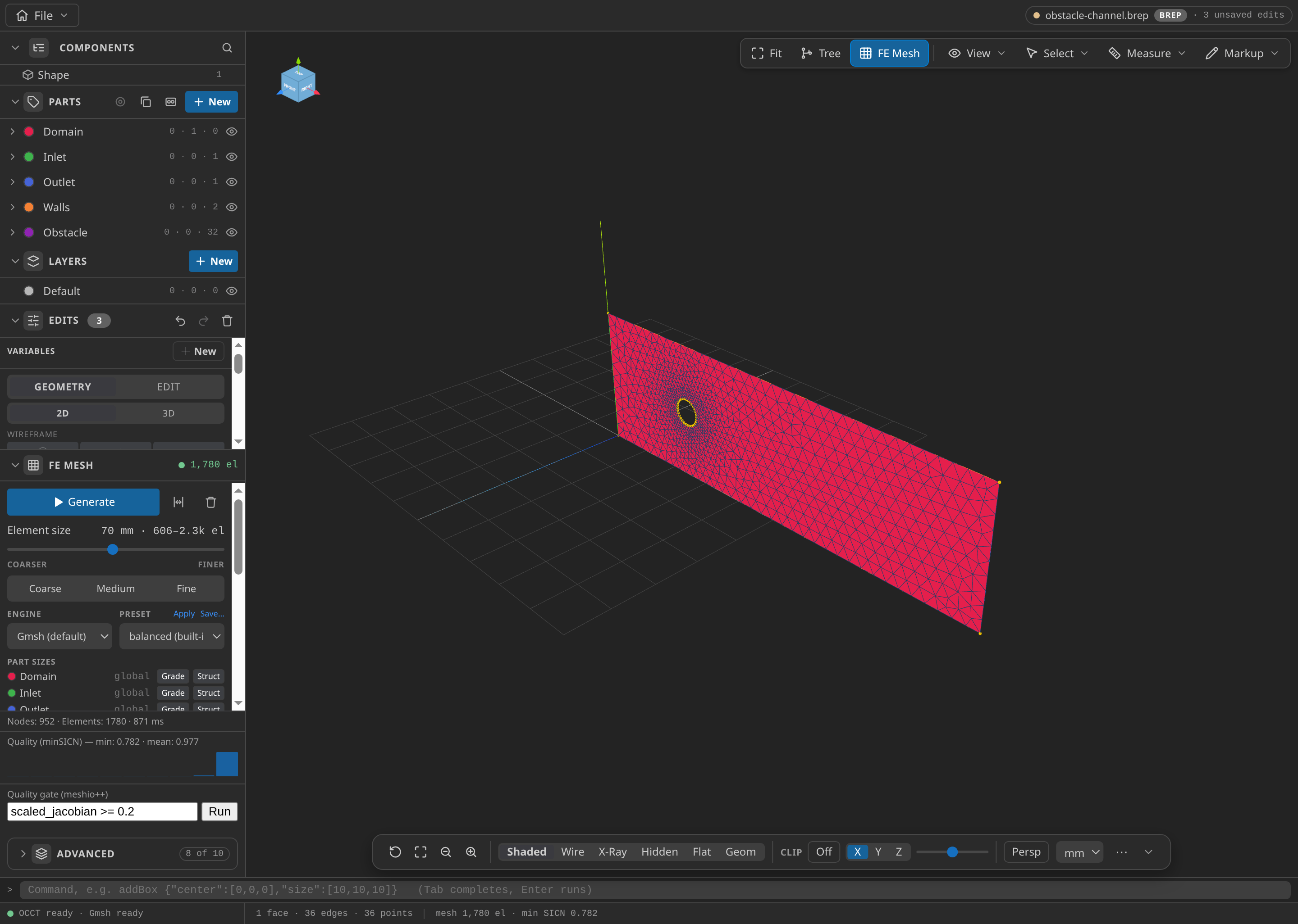
The CAD window after FE Mesh ▸ Generate: 952 nodes and 1,780 elements in this run, with the Parts panel open.

Configure the problemtype

5. Open mesh.mdpa in Post-Processing and select Fluid Dynamics. Enter the setup below.

Card	Item	Value
Materials	Domain	Newtonian 2D: density 1000 kg/m³, dynamic viscosity 0.6 Pa·s
Conditions	Inlet velocity on Inlet	0.1 m/s, direction +X, active from 0 s to the end
Conditions	Outlet pressure on Outlet	0, hydrostatic contribution off
Conditions	Slip wall on Walls; no-slip wall on Obstacle	slip; no-slip
Problem data	Strategy, Element, Time scheme	Monolithic, Classic VMS (legacy), Bossak (alpha −0.3, dynamic tau 1)
Problem data	Time stepping, step, start, end	Fixed step, 0.1 s, 0 s, 5 s
Problem data	Max iterations	20
Output	VTK	every step, ASCII, VELOCITY and PRESSURE

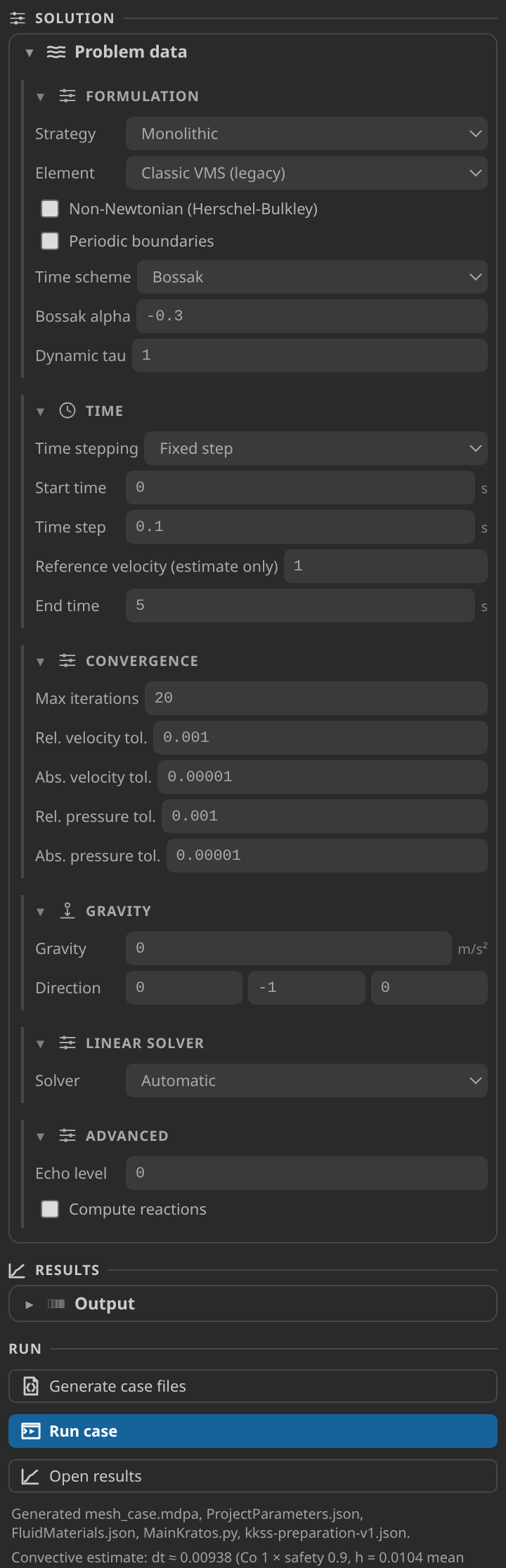
The Problem data card, with the convective estimate under the Run buttons.

The convective estimate uses the Reference velocity, which defaults to 1 m/s. At that default it reads about 0.009 s, ten times too small for this inlet. Enter 0.1 m/s explicitly. The estimate then reads about 0.09 s, so the 0.1 s step sits close to a Courant number of one.

Generate and inspect the case files

6. Click Generate case files. The status line lists mesh_case.mdpa, ProjectParameters.json, FluidMaterials.json, MainKratos.py and kkss-preparation-v1.json.

mesh_case.mdpa is written only when element names must change, and mesh.mdpa stays untouched. kkss-preparation-v1.json records the effective parameters and input hashes, so a run can be traced to its settings.

Run

7. In Settings → Simulation, point kratos.pythonPath at a Python environment that imports KratosMultiphysics and KratosFluidDynamicsApplication. Use the Home screen's Check environment action, then click Run case. To stop a run, use File ▸ Stop Kratos Run, which lets the driver finish the current step. The verification used Python 3.12.14, Kratos 10.4.3 and two OpenMP threads.

Inspect the results

8. Click Open results. In Field, choose VELOCITY or PRESSURE, and move the timeline through the 51 frames to t = 5 s. For the Field panel, timeline and plots, see Reading a Kratos result in KKSS.

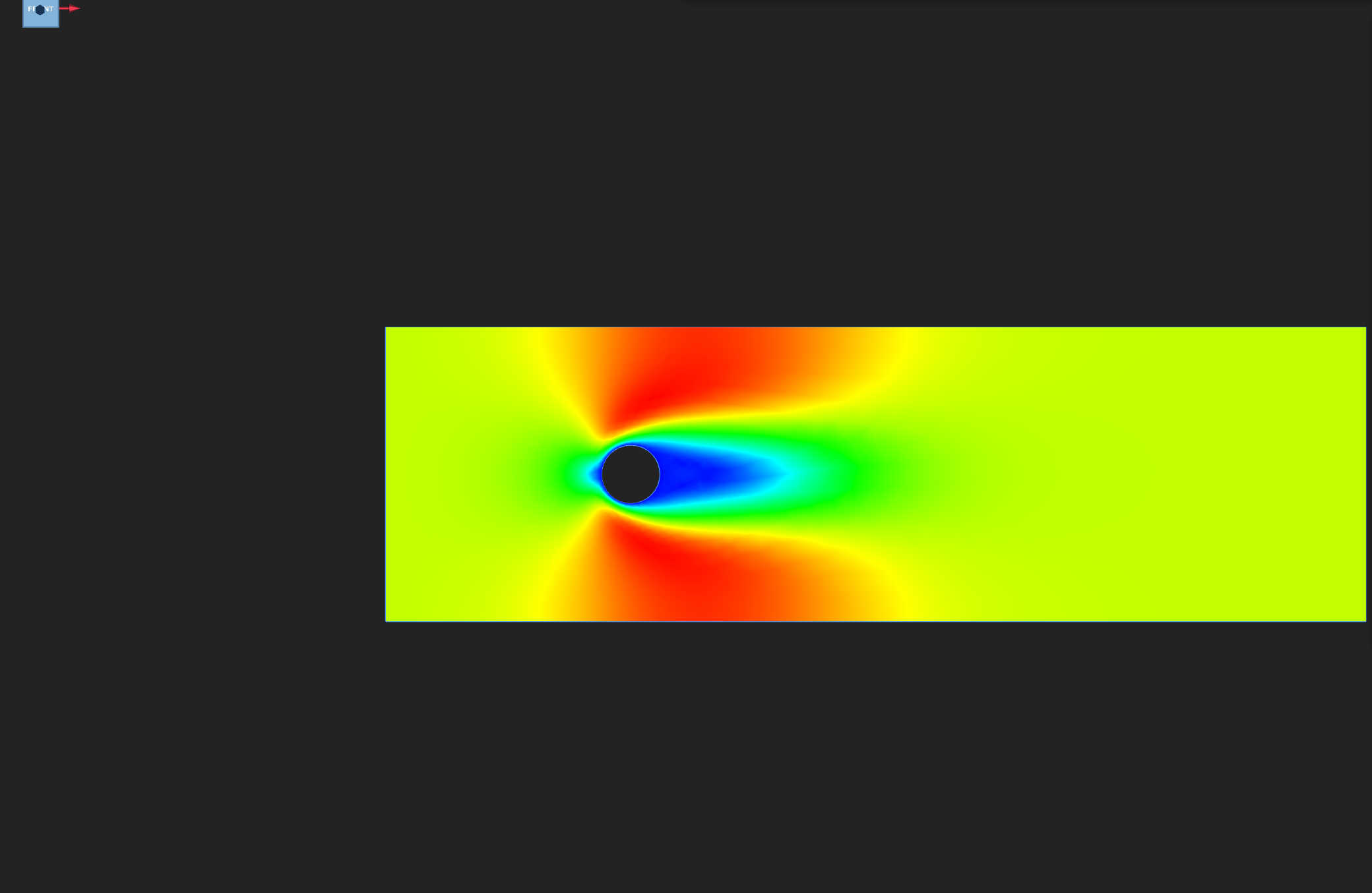
Velocity magnitude on the final frame, colour range 0 to about 0.14 m/s. Fast flow (red) passes the obstacle's sides, and the slow blue pocket behind it is the wake.

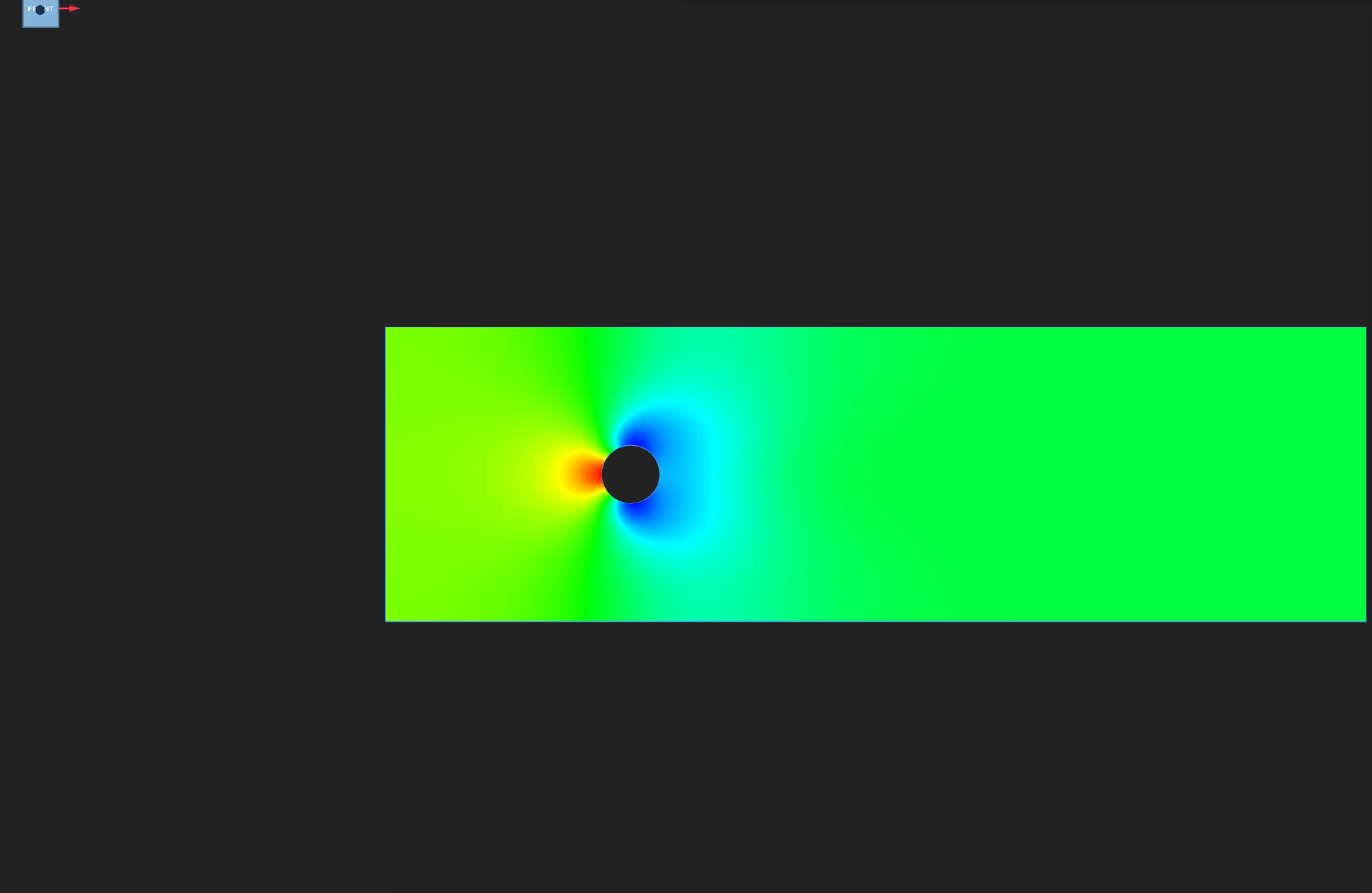
Pressure on the final frame, on the frame's own range of −7.23 to 9.28. Stagnation (red) is on the upstream face.

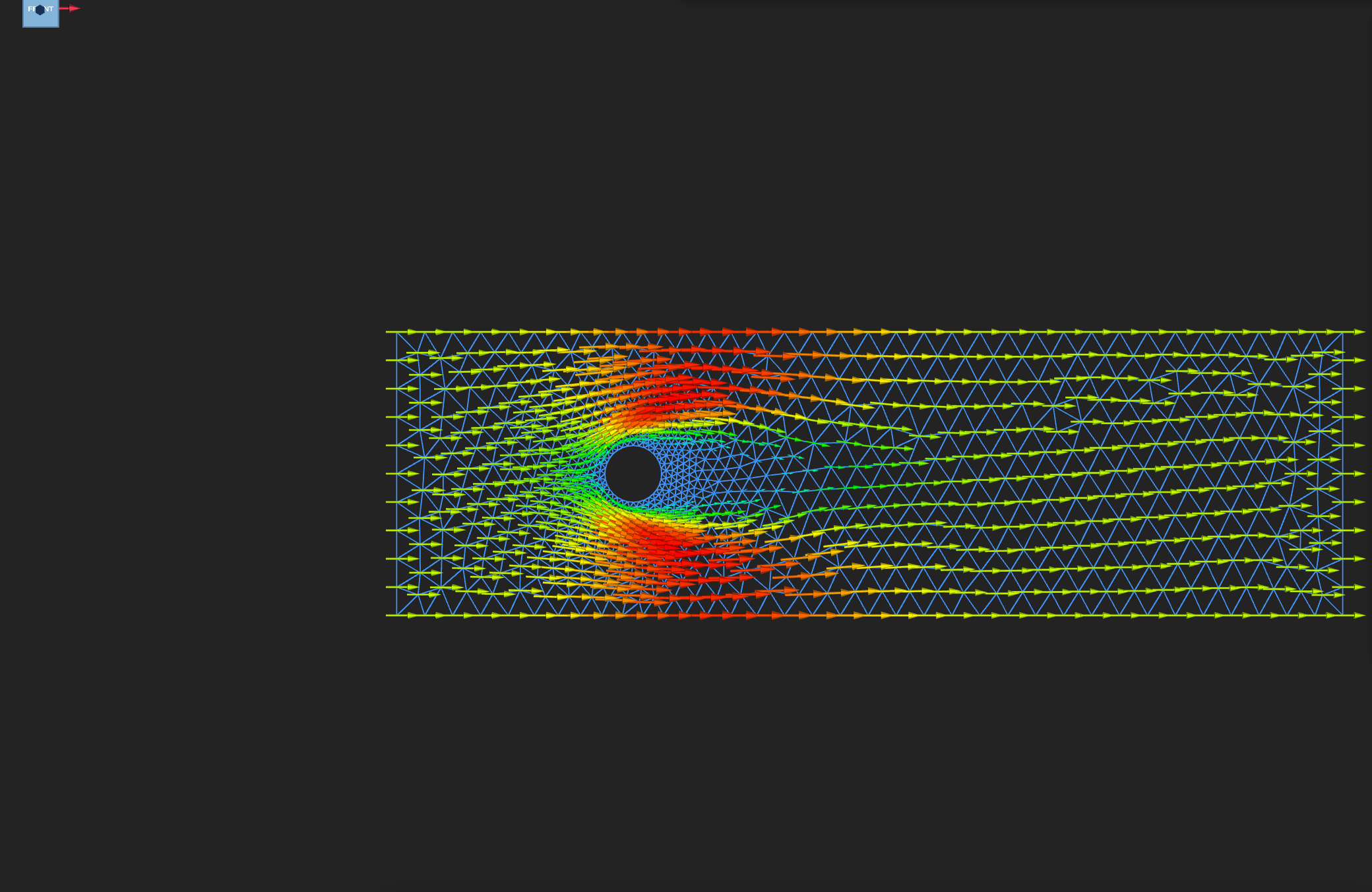
Quiver arrows of the final velocity. Look for flow turning around the obstacle.

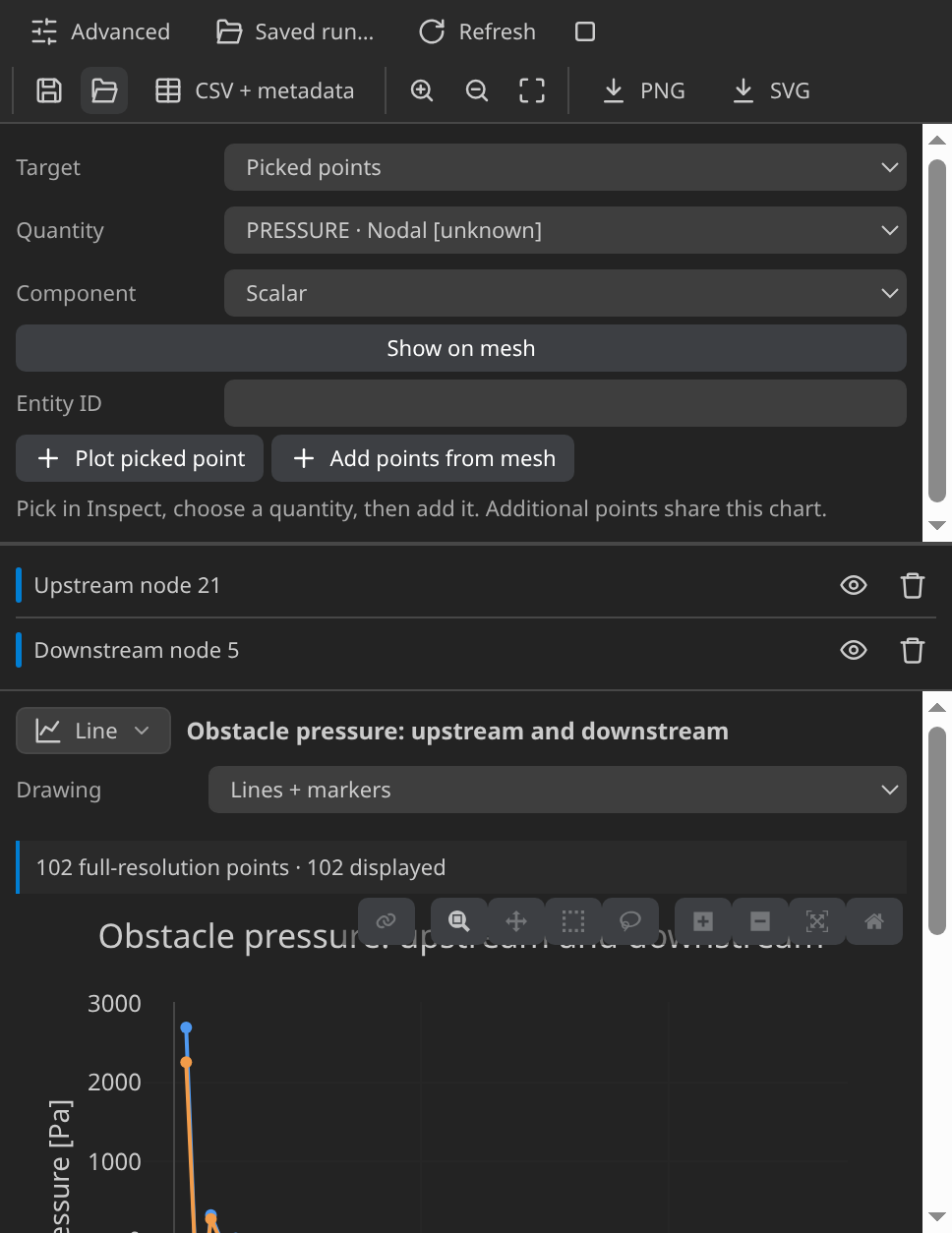
Pressure at two fixed probe nodes against time. Check that each trace has levelled off by t = 5 s.

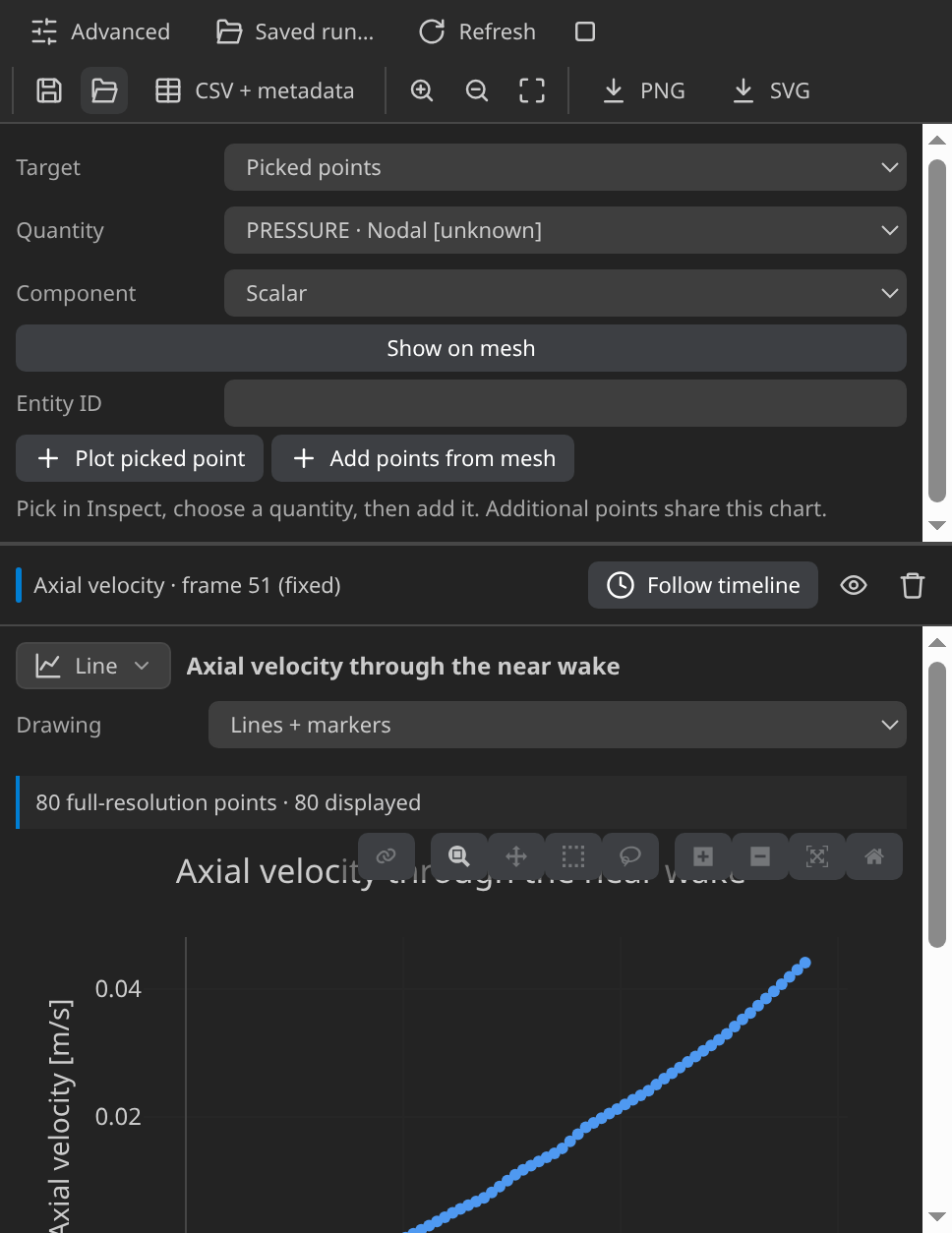
Axial velocity across the wake on the final frame. The verifier's deficit is the inlet speed minus the lowest near-wake value.

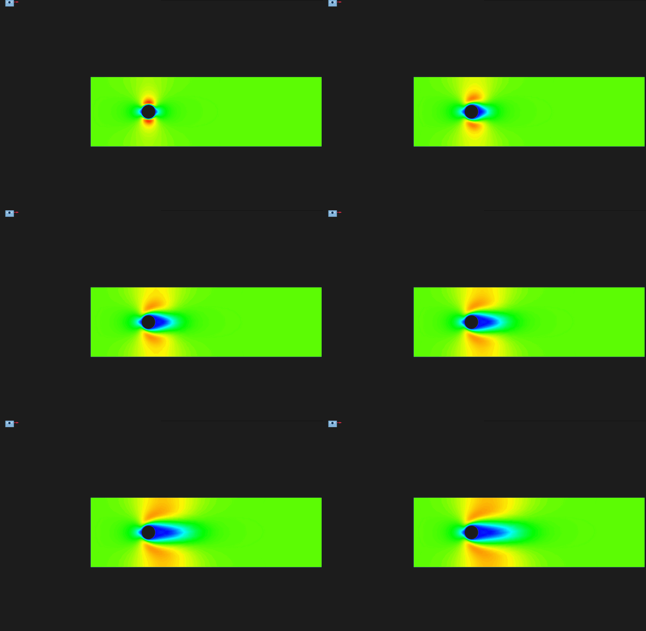
Velocity magnitude over steps 1 to 51 on a fixed 0–0.17 m/s scale.

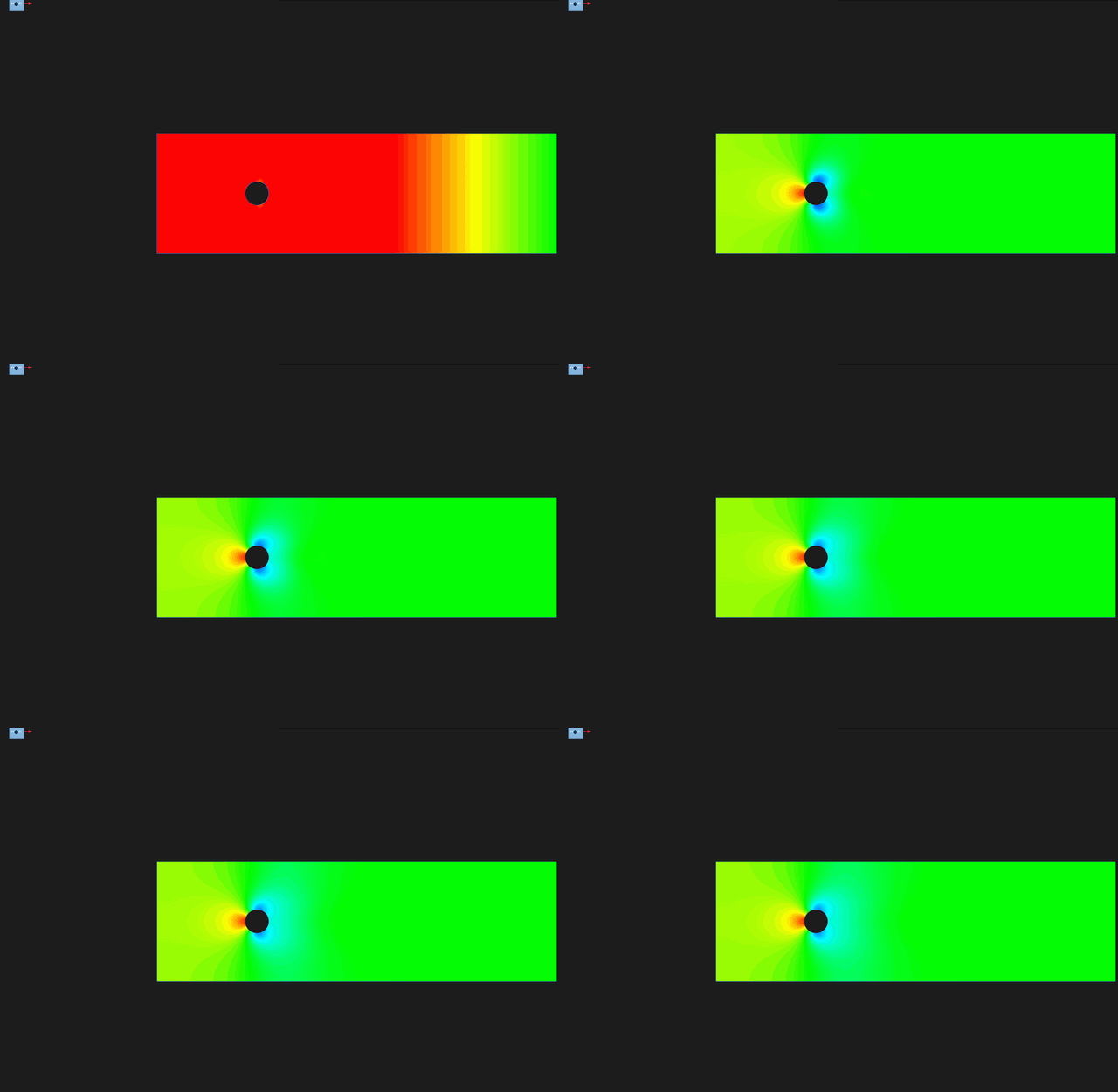
Pressure from step 5 to 51 on a fixed ±10 scale. The impulsive start would flatten the scale, so earlier steps are left out.

Verify

Verified with Python 3.12.14, Kratos 10.4.3, 2 OpenMP threads: 945 nodes and 1766 cells, 51 frames through t = 5.

Check	Measured	Limit
inlet_velocity_error_m_per_s	0	≤ 0.000001
outlet_pressure_error_Pa	0	≤ 0.000001
flux_imbalance_m2_per_s	2.399739e-10	≤ 0.001
inlet_flux_m2_per_s	0.06
outlet_flux_m2_per_s	0.06
obstacle_no_slip_speed_m_per_s	0	≤ 0.00002
near_wake_velocity_deficit_m_per_s	0.1047505	≥ 0.025
pressure_range_Pa	16.51441	≥ 0.05
reynolds_number	20
obstacle_boundary_nodes	32
wake_sample_nodes	20
minimum_near_wake_axial_velocity_m_per_s	-0.00475046
pressure_minimum_Pa	-7.234211
pressure_maximum_Pa	9.280196

These are tutorial checks with the tolerances shown, not formal solver certification.

The checks read the final frame and its sampled nodes. The inlet velocity matches 0.1 m/s in +X on every inlet node to within 10⁻⁶ m/s, and the outlet pressure is zero to the same tolerance. Integrated along the inlet, the streamwise velocity gives 0.060000002 m²/s per metre of depth, the inlet speed times the 0.6 m height. The outlet carries 0.06000000176 m²/s, an imbalance of 2.4 × 10⁻¹⁰ against a limit of 0.001. The 32 obstacle nodes measure zero speed.

The near-wake sample holds 20 nodes, between 1.5 and 5 obstacle radii behind the centre and within 0.35 radius of the centreline. Its deficit, 0.1 − (−0.00475) = 0.10475 m/s, clears its 0.025 limit, and the negative minimum shows reversed flow. The pressure range, from −7.23 to 9.28, clears its limit of 0.05.

The checks do not compare drag or lift with a reference, and the mesh is not refined for convergence. They confirm the setup at this resolution.

Troubleshooting

• Segmentation fault at the first step. BDF2 segfaults this build. Set the time scheme to Bossak.
• Import fails at run start. The environment lacks KratosFluidDynamicsApplication, or kratos.pythonPath points elsewhere.
• The estimate looks ten times too small. The reference velocity is still 1 m/s. Enter 0.1 m/s.

Variations to try

• Double the inlet speed to 0.2 m/s. Re doubles to 40.
• Divide the viscosity by ten. Re becomes 200, where the wake stops being steady, so expect a finer mesh and a shorter step.
• Try the turbulent case, or build your own plot.

Reproduce and download

The complete case is fluid case with its verification record: the CAD source, the generation setup, the generated case and SHA-256 provenance. Run MainKratos.py with Python 3.12.14 and Kratos 10.4.3 to reproduce the VTK timeline. Rerunning overwrites generated outputs.