Getting Started
This walkthrough builds a small graph and generates a Kratos configuration from it. It assumes the editor is running — see Installation — and open at http://localhost:8182.
The editor at a glance
When FlowGraph loads you see the toolbar across the top and an infinite, pannable canvas below.
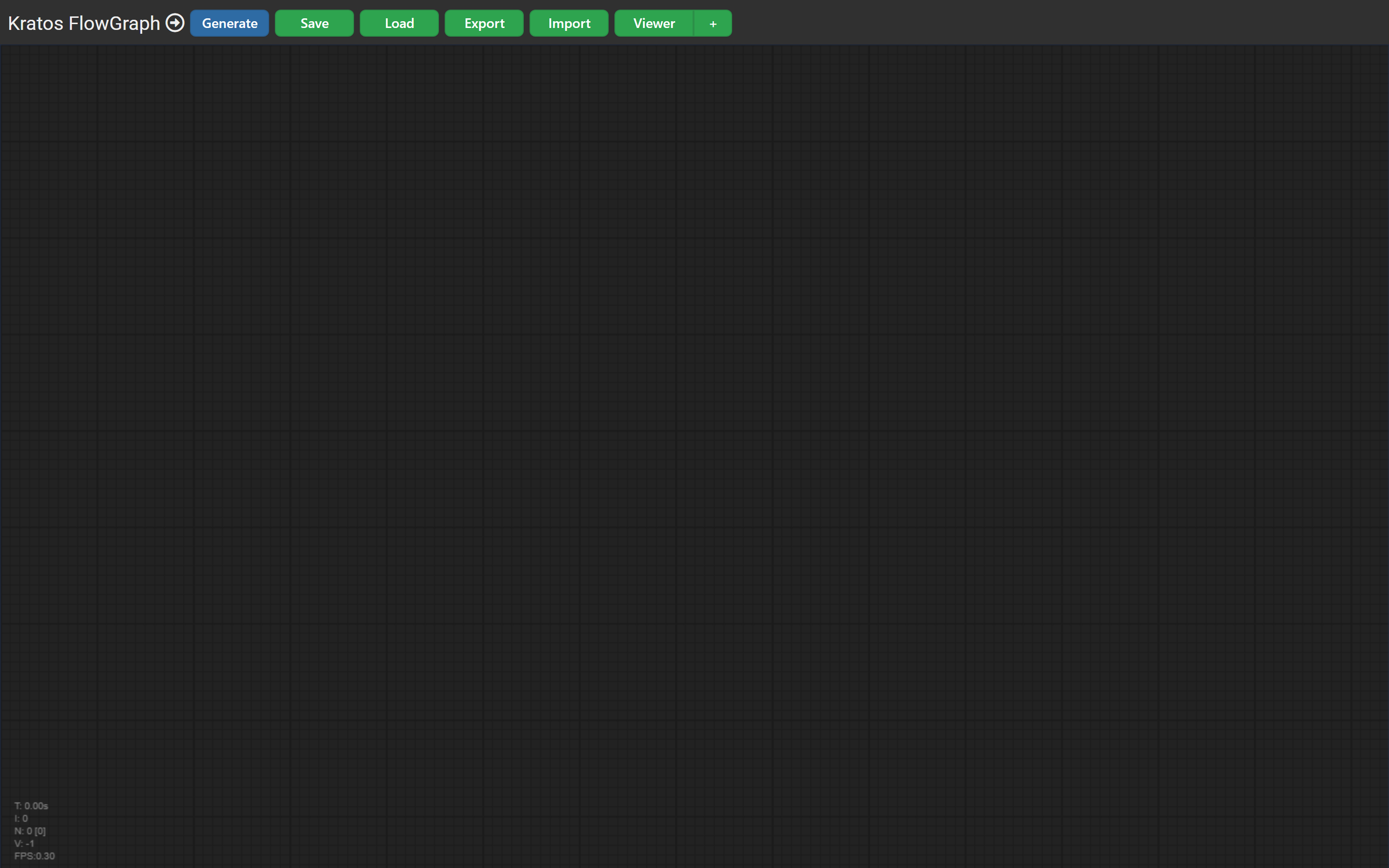
The toolbar buttons are covered in detail in The Toolbar. In short:
| Button | Action |
|---|---|
| Generate | Execute every node (onExecute) to compute the resulting JSON. |
| Save / Load | Download / restore the full graph as graph.json. |
| Export / Import | Save / restore only the currently selected nodes (a reusable "selection"). |
| Viewer | Toggle the live JSON side panel. |
| + | Add a JSONView node to the canvas. |
Add a node
Right-click anywhere on the canvas and choose Add Node. FlowGraph presents the node library grouped by category — Analysis stages, Solvers, Materials, Processes, Modelers, Model Parts, IO, and more.
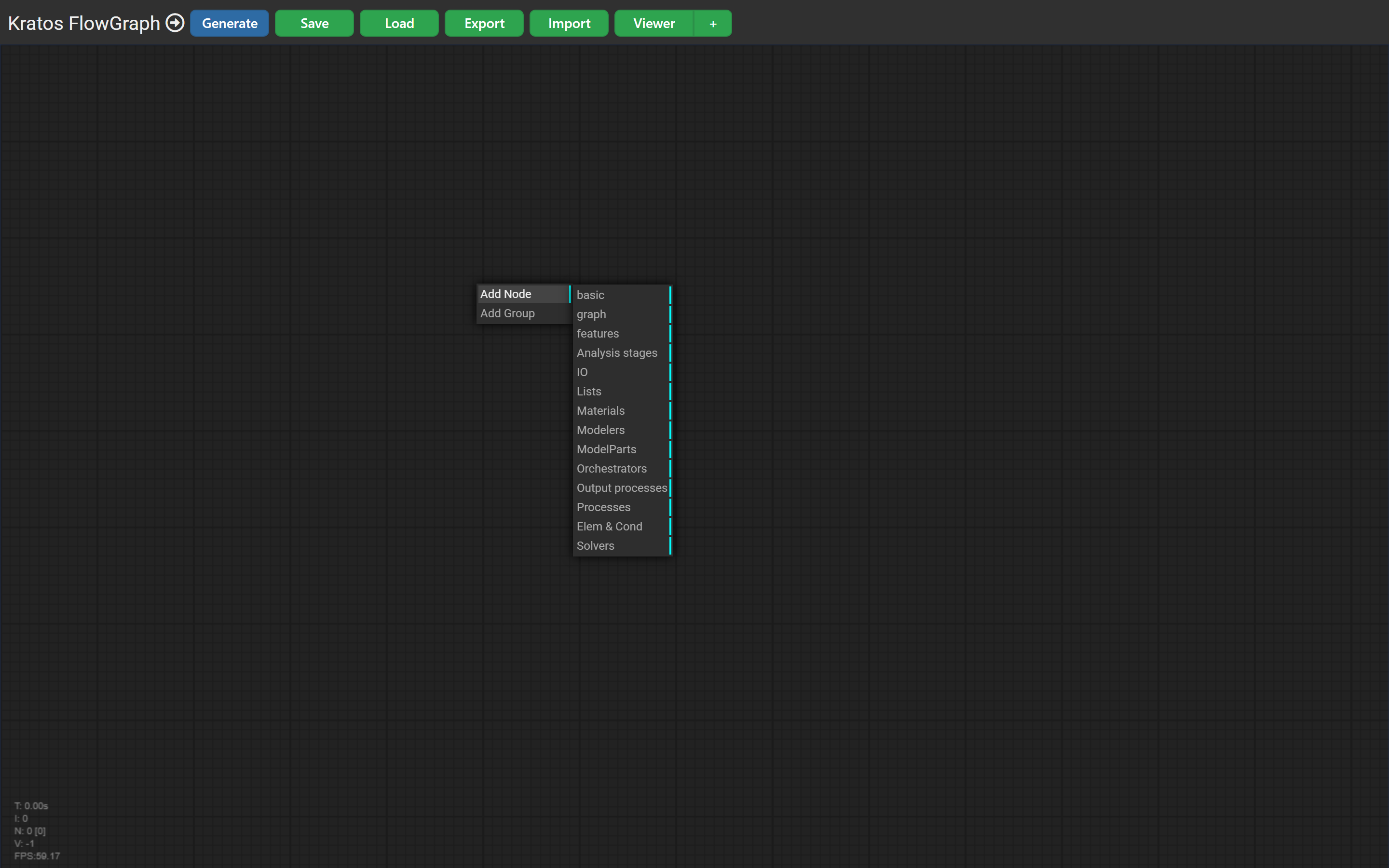
Navigate into a category and click a node to drop it on the canvas at the cursor position. You can also drag nodes around, and zoom with the scroll wheel.
Configure a node
Every node exposes widgets (its editable properties) and slots (its inputs on the left, outputs on the right). Constitutive-law material nodes are a good example of rich configuration — here a Small strain isotropic damage 3D node exposes its yield surface and material constants:
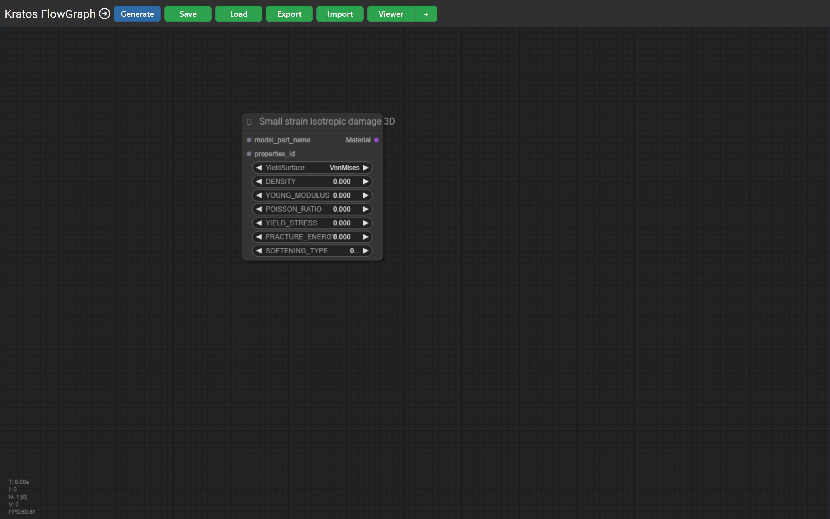
Click a widget to edit it: text fields open an input box, combos (◀ value ▶) cycle through allowed values, numbers can be dragged or typed. The available widgets change dynamically based on other choices (for example, selecting a yield surface reveals the relevant constants).
Connect nodes
Drag from an output slot (right side of a node) to a compatible input slot (left side of another node) to create a connection. Connections express how Kratos concepts reference each other: a solver takes a linear solver and model-import settings, an analysis stage takes a solver, problem data, processes and outputs, and so on.
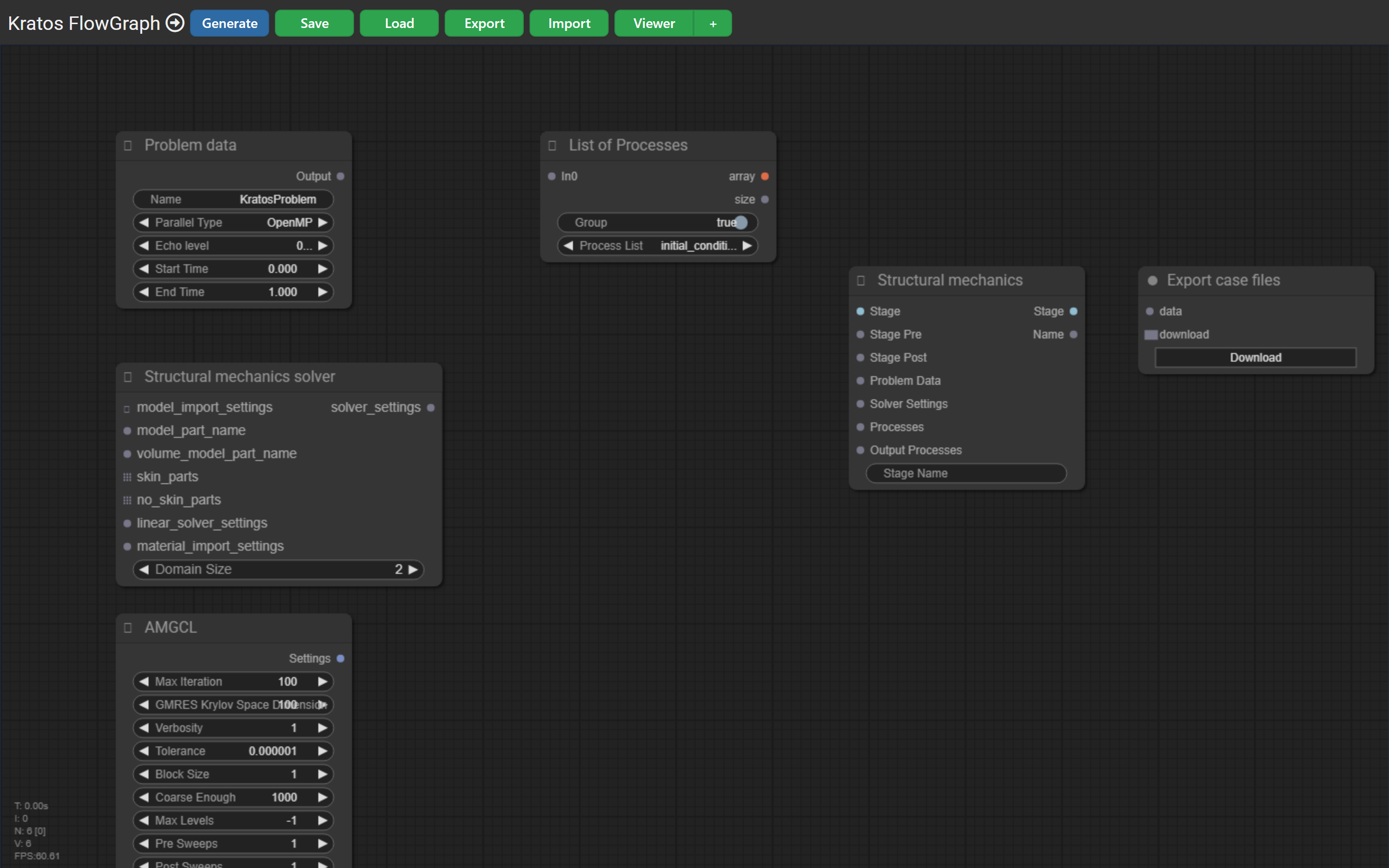
A typical structural graph wires Problem Data, a Structural Mechanics Solver (fed by a linear solver such as AMGCL), a List of Processes and an Analysis Stage into an Export case files node.
See the generated JSON
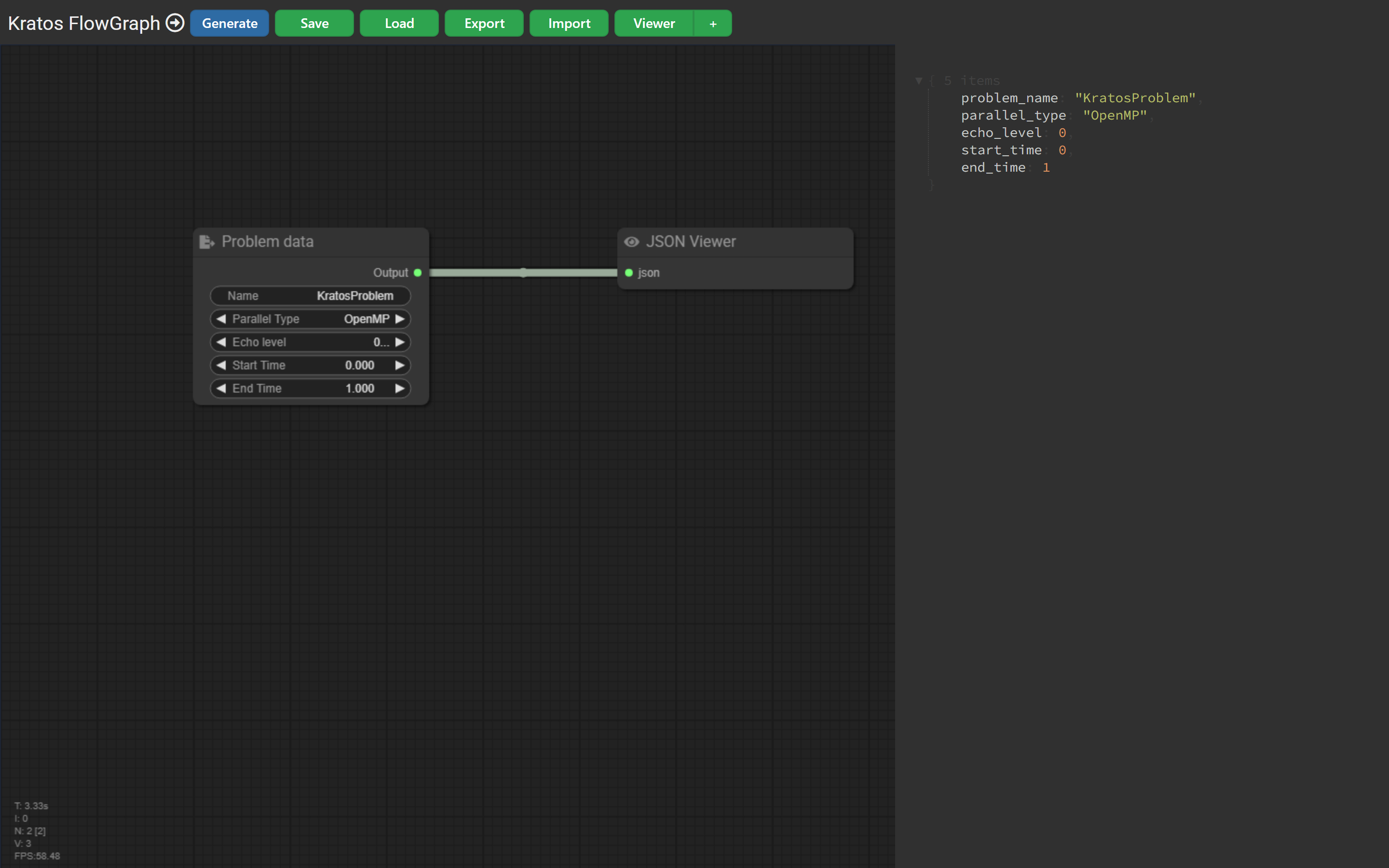
Click Generate to run the graph, then toggle Viewer to open the side panel. It renders the JSON produced by the currently connected nodes as you work. Here a Problem Data node feeds a JSON Viewer node, and the panel shows the resulting problem_data block:
Export a runnable case
When your graph is complete, use an Export case files (IO/DownloadProblem) node to download a case.zip containing ProjectParameters.json and the material files — ready to run with Kratos. See Exporting a Case for the details.
Where to go next
- The Toolbar — every toolbar action explained.
- Importing ProjectParameters — turn an existing Kratos case back into a graph.
- Node Reference — the full catalogue of node types.